Duality, Wasserstein-1, and Semi-discrete OT
Dual potentials, Lipschitz witnesses, Laguerre cells, and quantization algorithms.
Gabriel Peyré
CNRS and École normale supérieure, PSL Université
Optimal Transport for Machine Learners
Why duality matters
Kantorovich relaxation turns OT into a linear program. Its dual exposes functions rather than couplings.
This is useful because dual potentials:
- certify optimality,
- define gradients of OT losses,
- produce W_1 witnesses and GAN critics,
- drive semi-discrete algorithms.
source: \alpha,x,atarget: \beta,y,bplan/map: \pi,P,T
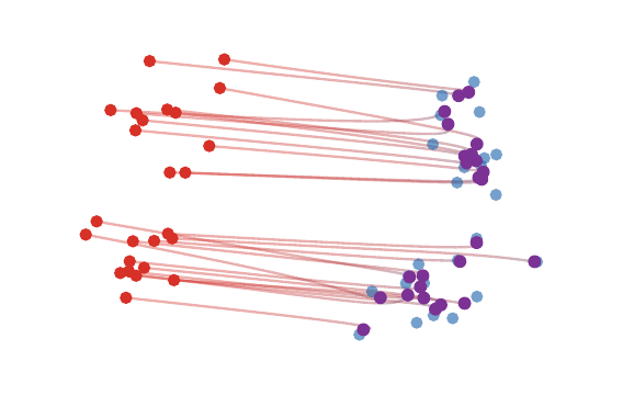
Dual potentials touch the cost on transported pairs.
Roadmap: duality
1. Duality
2. Wasserstein-1 and IPMs
3. Semi-discrete OT
4. Quantization
5. Learning links
Discrete primal and dual
Discrete Kantorovich primal. For a\in\Sigma_n, b\in\Sigma_m and C\in\mathbb R^{n\times m},
\mathcal L_C(\textcolor{#c7372f}{a},\textcolor{#226db4}{b})=
\min_{\textcolor{#7c5bbd}{P}\geq0}
\langle C,\textcolor{#7c5bbd}{P}\rangle
\quad\text{s.t.}\quad
\textcolor{#7c5bbd}{P}\mathbb 1_m=\textcolor{#c7372f}{a},
\quad \textcolor{#7c5bbd}{P}^\top\mathbb 1_n=\textcolor{#226db4}{b}.
Discrete dual.
\mathcal L_C(\textcolor{#c7372f}{a},\textcolor{#226db4}{b})=
\max_{f\in\mathbb R^n,\ g\in\mathbb R^m}
\langle f,\textcolor{#c7372f}{a}\rangle+\langle g,\textcolor{#226db4}{b}\rangle
\quad\text{s.t.}\quad
f_i+g_j\leq C_{i,j}.
Lagrangian derivation
The Lagrangian of the primal is
\langle C,\textcolor{#7c5bbd}{P}\rangle+
\langle f,\textcolor{#c7372f}{a}-\textcolor{#7c5bbd}{P}\mathbb 1_m\rangle+
\langle g,\textcolor{#226db4}{b}-\textcolor{#7c5bbd}{P}^\top\mathbb 1_n\rangle.
Minimizing over P\geq0 gives a finite value if and only if
C_{i,j}-f_i-g_j\geq0\quad\forall i,j.
This yields the dual constraints f_i+g_j\leq C_{i,j}.
Complementary slackness
Primal-dual contact. If P and (f,g) are optimal, then
\textcolor{#7c5bbd}{P}_{i,j}>0\quad\Longrightarrow\quad f_i+g_j=C_{i,j}.
Mass is transported only on the contact set of the dual constraint.
Discrete dual witnesses
Dual variables are not just algebraic multipliers: they are certificates explaining which transport edges can be active.
Live panel: discrete dual potentials
Dual certificates identify the active transport pairs.
Continuous duality
Kantorovich duality. On Polish spaces, for a lower-semicontinuous cost c bounded from below,
\mathcal L_c(\textcolor{#c7372f}{\alpha},\textcolor{#226db4}{\beta})
=
\sup_{f,g}
\int f\,d\textcolor{#c7372f}{\alpha}+
\int g\,d\textcolor{#226db4}{\beta}
\quad\text{s.t.}\quad
f(\textcolor{#c7372f}{x})+g(\textcolor{#226db4}{y})\leq c(\textcolor{#c7372f}{x},\textcolor{#226db4}{y}).
Here “Polish” means complete and separable after choosing a compatible metric. This is the infinite-dimensional analogue of the finite LP dual.
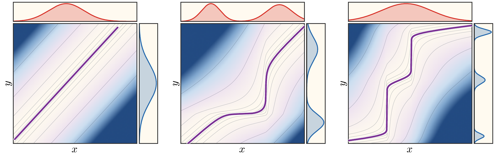
Continuous potentials
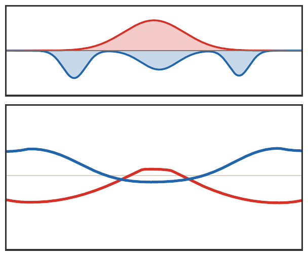
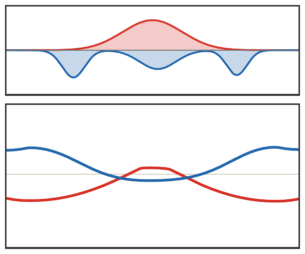
For quadratic cost in one dimension, optimal potentials encode the monotone transport map through their derivatives.
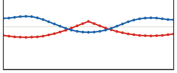
Live panel: continuous Kantorovich potentials
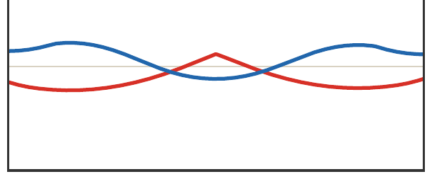
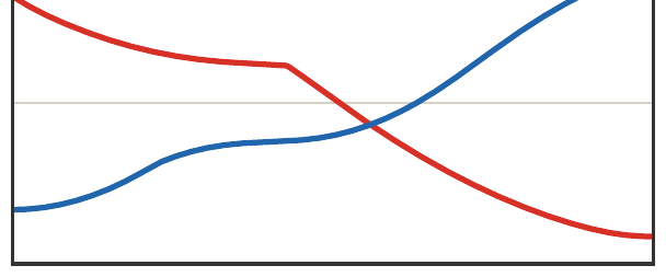
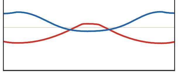
In one dimension, the contact condition can be read directly from the potential curves.
Reduced dual value
The c-transform removes one dual variable:
\mathcal L_c(\textcolor{#c7372f}{\alpha},\textcolor{#226db4}{\beta})
=
\sup_f
\left\{
\int f\,d\textcolor{#c7372f}{\alpha}+\int f^c\,d\textcolor{#226db4}{\beta}
\right\}.
In the discrete case this is
\mathcal L_C(\textcolor{#c7372f}{a},\textcolor{#226db4}{b})=
\max_{f\in\mathbb R^n}
\left\{
\langle f,\textcolor{#c7372f}{a}\rangle+\langle f^C,\textcolor{#226db4}{b}\rangle
\right\},
\qquad
f^C_j=\min_i(C_{i,j}-f_i).
This is the formula behind alternating c-transform updates.
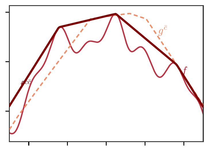
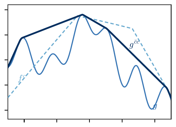
c-concavity
Reduction to one potential. At optimum one can impose
g=f^c,
\qquad
f=g^{\bar c}.
Thus dual potentials are fixed points of alternating c-transforms, up to non-uniqueness.
Interactive: changing the cost exponent
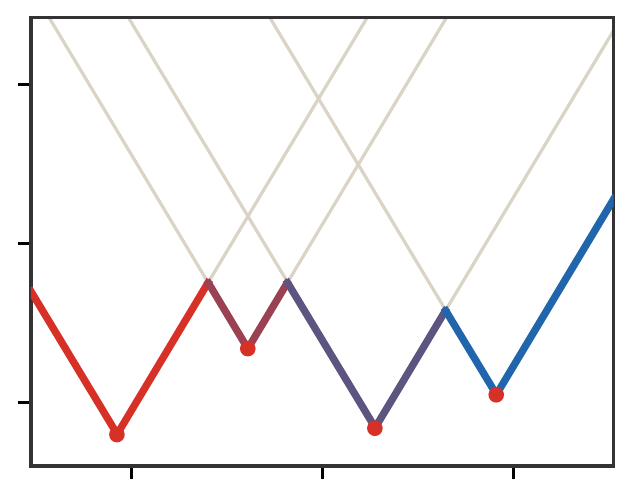
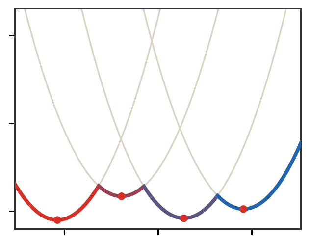
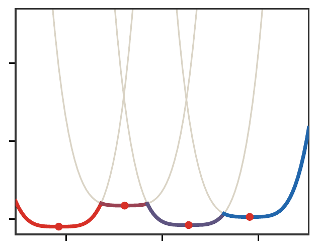
The c-transform closes a potential under the constraint f(\textcolor{#c7372f}{x})+g(\textcolor{#226db4}{y})\leq c(\textcolor{#c7372f}{x},\textcolor{#226db4}{y}). Changing the cost exponent changes the envelope selected by the dual constraint.
Here c_p(\textcolor{#c7372f}{x},\textcolor{#226db4}{y})=|\textcolor{#c7372f}{x}-\textcolor{#226db4}{y}|^p and the slider controls p.
Existence of dual optimizers
Lipschitz compactness principle. When the cost is Lipschitz on compact supports, optimal potentials can be chosen uniformly Lipschitz. Arzela-Ascoli compactness then yields an optimizer.
This proof idea is important because the dual problem is over functions, not finite-dimensional vectors.
Roadmap: Wasserstein-1 and integral probability metrics
1. Duality
2. Wasserstein-1 and IPMs
3. Semi-discrete OT
4. Quantization
5. Learning links
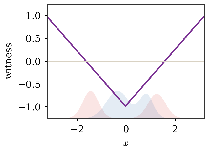
Wasserstein-1 as a norm
Norm viewpoint. On signed measures with zero total mass,
\|\textcolor{#c7372f}{\alpha}-\textcolor{#226db4}{\beta}\|_{W_1}:=W_1(\textcolor{#c7372f}{\alpha},\textcolor{#226db4}{\beta})
is a norm whenever the ground metric is fixed.
This places W_1 among dual norms defined by classes of test functions.
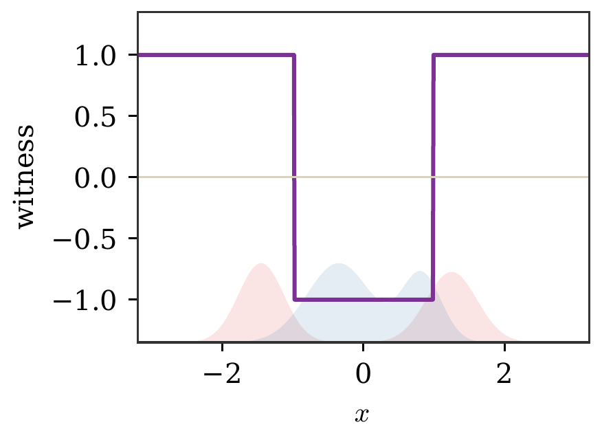
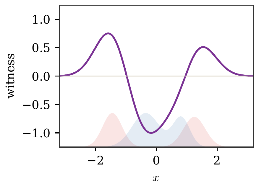
Integral probability metrics
Integral probability metric. Given a symmetric class of test functions \mathcal F,
D_\mathcal F(\textcolor{#c7372f}{\alpha},\textcolor{#226db4}{\beta})=
\sup_{f\in\mathcal F}\int f\,d(\textcolor{#c7372f}{\alpha}-\textcolor{#226db4}{\beta}).
Examples include total variation, Wasserstein-1, bounded-Lipschitz distances, and MMDs.
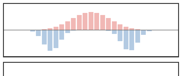
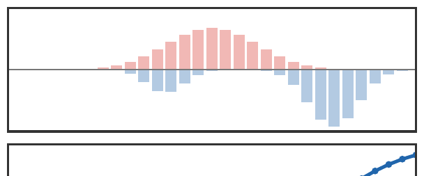
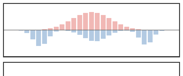
Live panel: integral probability metrics
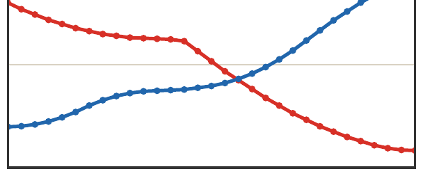
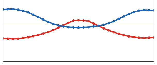
Changing the witness class changes the geometry of the discrepancy.
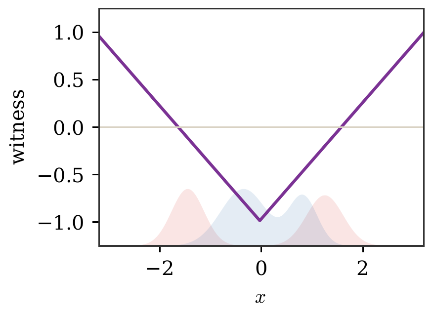
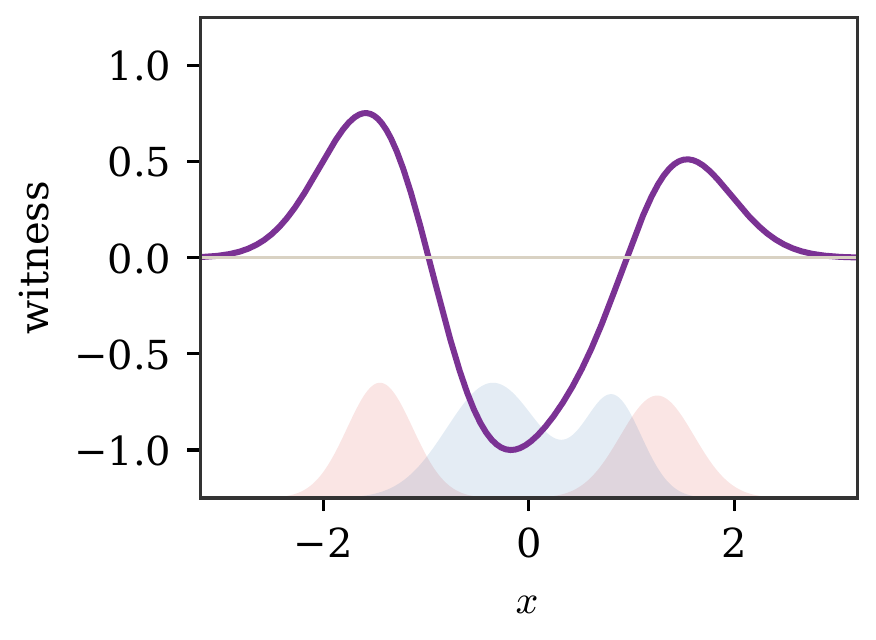
Dual witnesses compared
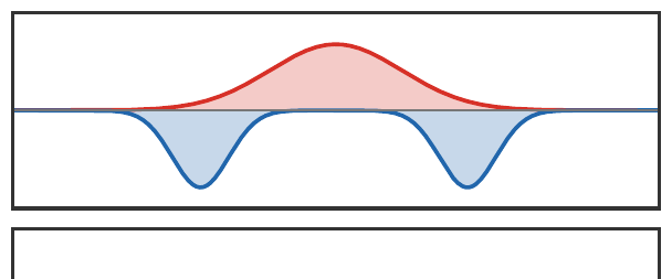
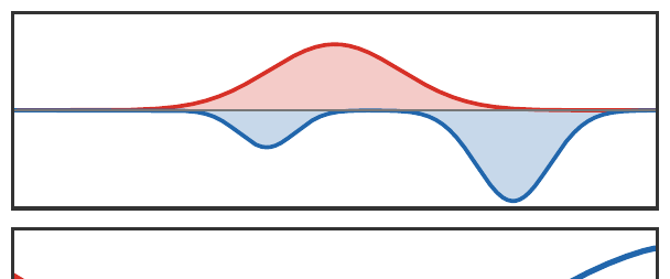
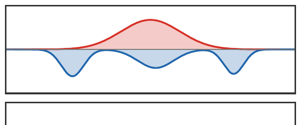
Different function classes produce different witnesses and therefore different notions of discrepancy.
Live panel: witness constraints
The same signed mass can be tested by very different admissible witnesses.
Wasserstein-1 on Euclidean domains
For smooth f on Euclidean domains, \operatorname{Lip}(f)\leq1 is equivalent to
\|\nabla f(x)\|\leq1.
This connects W_1 to Beckmann’s continuous flux formulation:
W_1(\textcolor{#c7372f}{\alpha},\textcolor{#226db4}{\beta})=
\min_{\textcolor{#7c5bbd}{m}}\int \|\textcolor{#7c5bbd}{m}(\textcolor{#c7372f}{x})\|\,d\textcolor{#c7372f}{x}
\quad\text{s.t.}\quad
\operatorname{div}\textcolor{#7c5bbd}{m}=\textcolor{#c7372f}{\alpha}-\textcolor{#226db4}{\beta}.
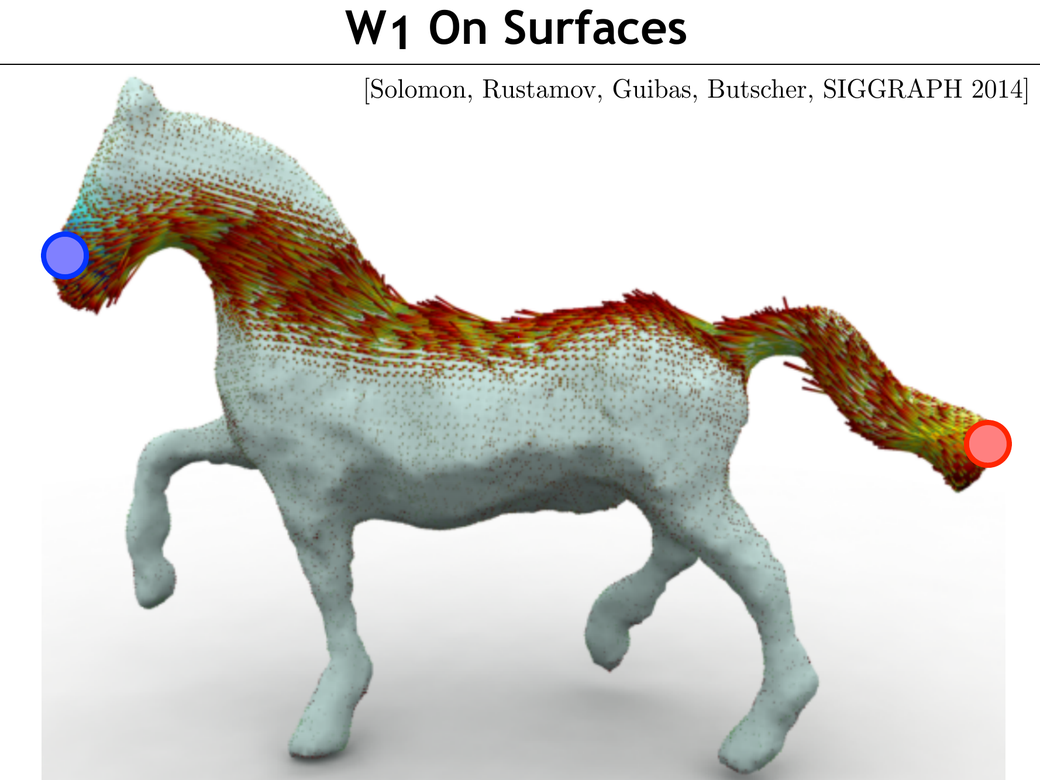
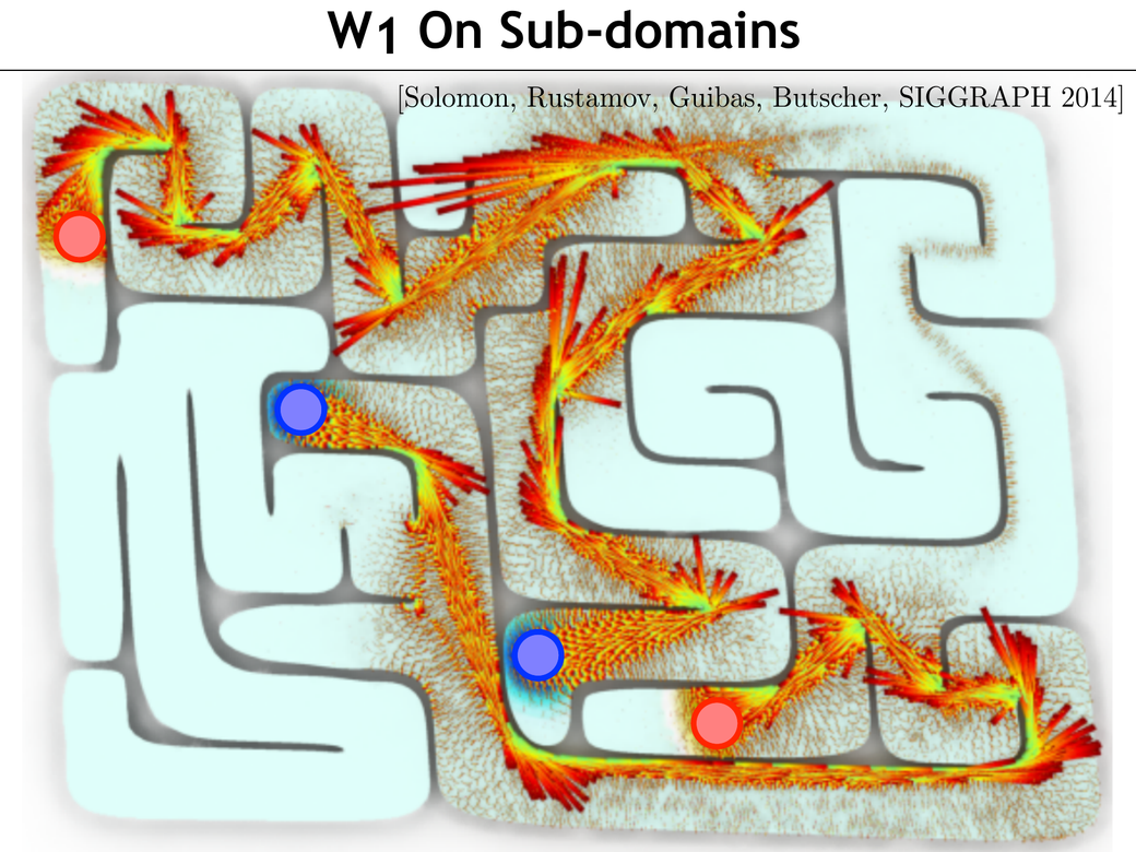
W1 on surfaces and subdomains
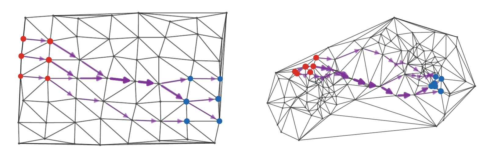
The same Beckmann idea extends beyond flat Euclidean grids by replacing gradients and divergence with their geometric counterparts.
Geometric message. On meshes, surfaces, or subdomains, W_1 can be computed as a flow constrained by the geometry. Graph discretizations are the simplest finite-dimensional version of this idea.
This is the setting of surface and subdomain W_1 solvers used in geometry processing, including the Solomon-Rustamov-Guibas-Butscher line of work. Graph flows are the simplest discrete proxy for this geometric formulation.
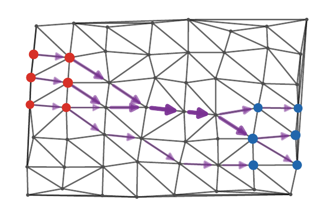
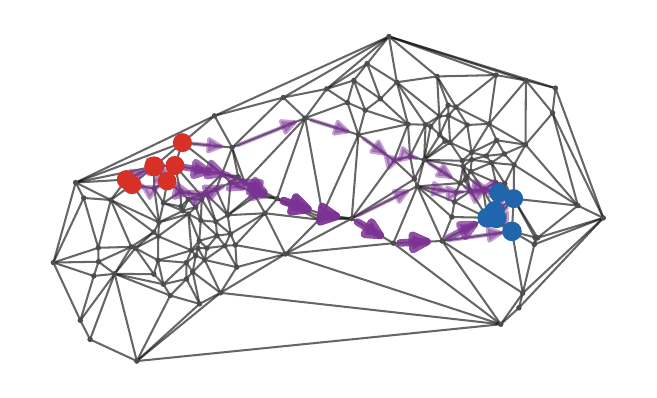
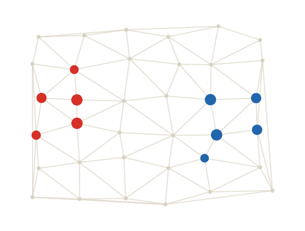
Wasserstein-1 on graphs
On a graph, the Beckmann formulation becomes a sparse network-flow problem over edges:
\min_{\textcolor{#7c5bbd}{q}}\sum_{e} w_e|\textcolor{#7c5bbd}{q_e}|
\quad\text{s.t.}\quad
D\textcolor{#7c5bbd}{q}=\textcolor{#c7372f}{a}-\textcolor{#226db4}{b}.
Here D is the signed vertex-edge incidence matrix and \textcolor{#7c5bbd}{q_e} is the oriented mass flux on edge e.
This can be much smaller than a full pairwise Kantorovich LP.
Live panel: graph Beckmann transport
The graph formulation turns W1 into a network flow problem.
Graph flow visualization
The edge flow is the sparse object that transports positive mass to negative mass through the graph geometry.
WGAN viewpoint
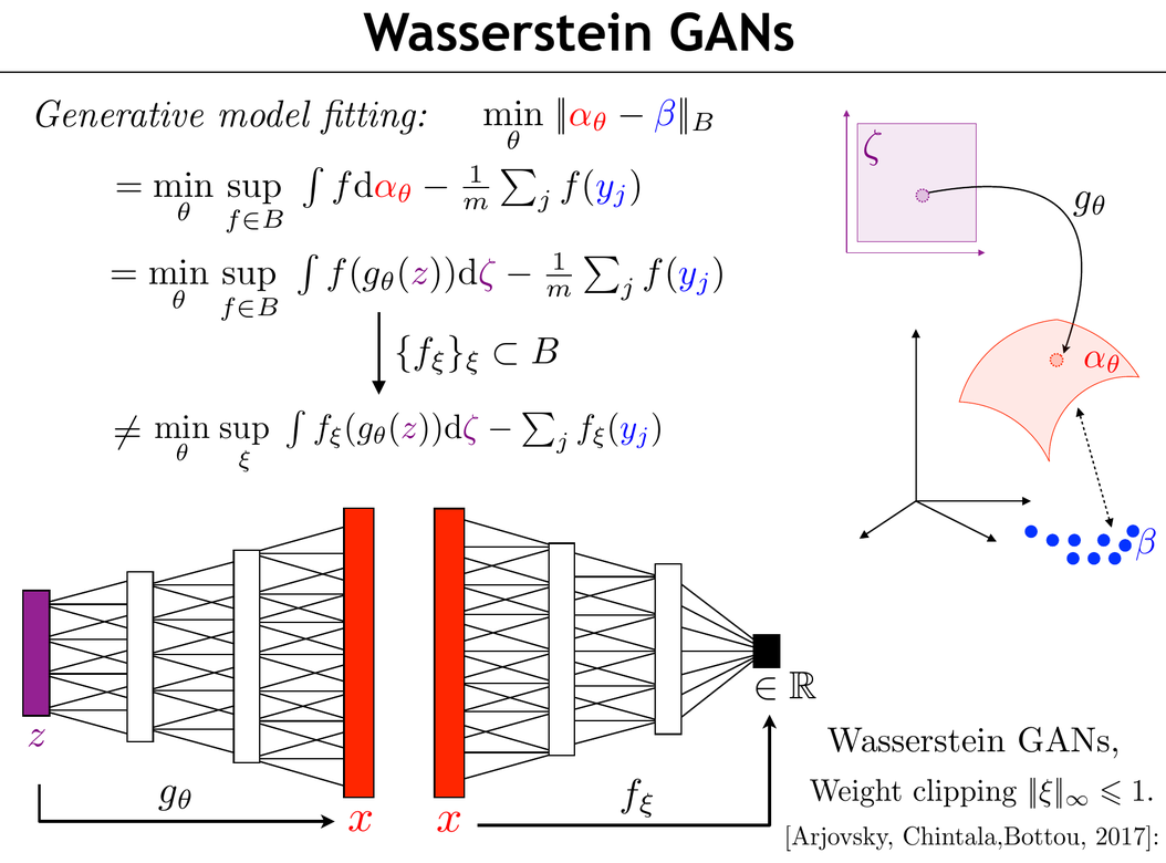
Example: Wasserstein GAN. A generator g_\theta can be trained by minimizing
\min_\theta W_1(\textcolor{#c7372f}{(g_\theta)_\#\zeta},\textcolor{#226db4}{\beta})
=
\min_\theta\sup_{\operatorname{Lip}(f)\leq1}
\mathbb E f(\textcolor{#c7372f}{g_\theta(Z)})-\mathbb E f(\textcolor{#226db4}{Y}).
The discriminator is a parametrized approximation of a 1-Lipschitz Kantorovich potential.
This is the machine-learning face of Kantorovich-Rubinstein duality.
Roadmap: semi-discrete OT
1. Duality
2. Wasserstein-1 and IPMs
3. Semi-discrete OT
4. Quantization
5. Learning links
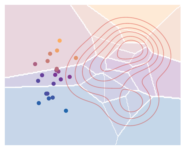
Semi-discrete setting
Semi-discrete OT. Let \alpha be a continuous probability measure on \mathbb R^d and
\textcolor{#226db4}{\beta}=\sum_{j=1}^m b_j\delta_{\textcolor{#226db4}{y_j}}
be discrete. For quadratic cost, one seeks a partition of the source domain whose cells have masses b_j.
The unknown is not a full coupling matrix but a weighted spatial partition.
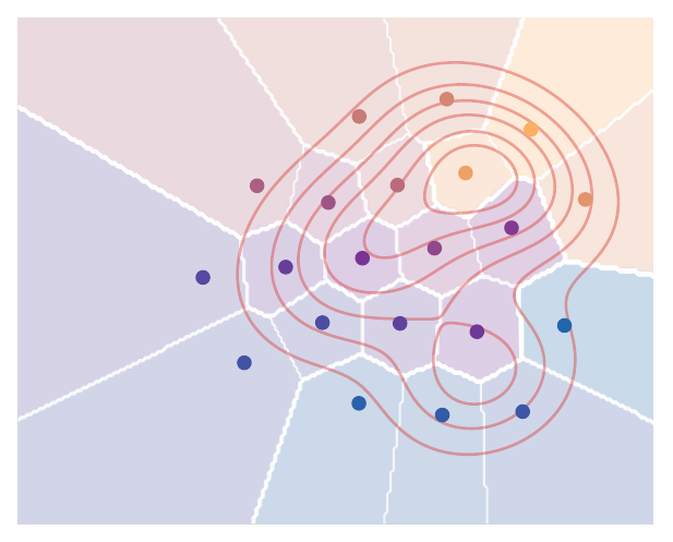
Laguerre cells
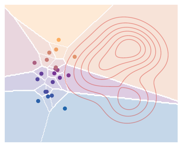
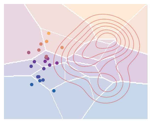
Laguerre cell. For target sites y_j and weights g_j, the cell associated with j is
L_j(g)=\{\textcolor{#c7372f}{x}: \|\textcolor{#c7372f}{x}-\textcolor{#226db4}{y_j}\|^2-g_j\leq \|\textcolor{#c7372f}{x}-\textcolor{#226db4}{y_k}\|^2-g_k\quad\forall k\}.
The semi-discrete map sends every x\in L_j(g) to y_j. Optimal weights are characterized by the mass constraints
\textcolor{#c7372f}{\alpha}(L_j(g))=\textcolor{#226db4}{b_j},\qquad j=1,\ldots,m.
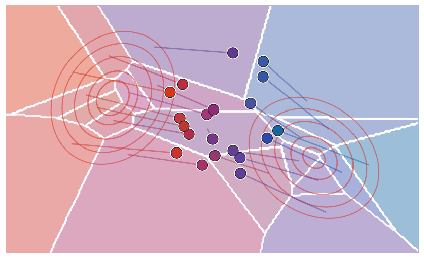
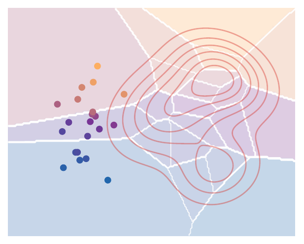
Live panel: Laguerre cells and dual weights
Changing a target weight geometrically expands or shrinks its cell.
Power diagrams
Voronoi cells become Laguerre cells when weights are introduced. The weights tune cell masses.
Interactive: one weight changes one cell
Changing g_j shifts the additive power distance
\|\textcolor{#c7372f}{x}-\textcolor{#226db4}{y_j}\|^2-g_j.
Increasing g_j makes site j more attractive and expands its Laguerre cell.
Semi-discrete dual
For quadratic cost, the dual can be written as a concave maximization over weights:
\max_{g\in\mathbb R^m}
\int \min_j\big(\|\textcolor{#c7372f}{x}-\textcolor{#226db4}{y_j}\|^2-g_j\big)\,d\textcolor{#c7372f}{\alpha}(\textcolor{#c7372f}{x})
+
\sum_{j=1}^m \textcolor{#226db4}{b_j} g_j.
Gradient. The gradient component is
\frac{\partial}{\partial g_j}=\textcolor{#226db4}{b_j}-\textcolor{#c7372f}{\alpha}(L_j(g)).
Thus dual ascent balances Laguerre cell masses.
Hessian and Newton structure
The reference semi-discrete solver uses the fact that the dual has an explicit sparse Hessian. If \textcolor{#c7372f}{\alpha}=\rho(x)\,dx and cells L_i(g) and L_j(g) share a facet
F_{i,j}=L_i(g)\cap L_j(g),
then for i\neq j,
\frac{\partial\,\textcolor{#c7372f}{\alpha}(L_i(g))}{\partial g_j}
=
-\frac{1}{2\|\textcolor{#226db4}{y_i}-\textcolor{#226db4}{y_j}\|}
\int_{F_{i,j}}\rho(x)\,d\mathcal H^{d-1}(x),
and the diagonal is chosen so rows sum to zero:
\frac{\partial\,\textcolor{#c7372f}{\alpha}(L_i(g))}{\partial g_i}
=-\sum_{j\neq i}
\frac{\partial\,\textcolor{#c7372f}{\alpha}(L_i(g))}{\partial g_j}.
Thus the Hessian of the concave dual has positive off-diagonal entries and negative diagonal row sums. Newton or quasi-Newton methods exploit the adjacency graph of the Laguerre diagram rather than a dense coupling matrix.
Weight descent as mass balancing
The algorithm updates the weights until every cell has the prescribed mass.
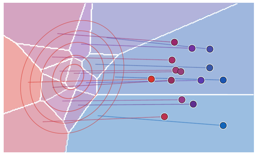
Semi-discrete examples
Coloring makes the spatial map visible: each source cell is sent to one target atom.
Practical optimization
Semi-discrete dual ascent. Input: source density \alpha, target sites y_j, target masses b_j.
Initialize weights g.
Repeat:
L_j(g)=\{\textcolor{#c7372f}{x}: \|\textcolor{#c7372f}{x}-\textcolor{#226db4}{y_j}\|^2-g_j\leq \|\textcolor{#c7372f}{x}-\textcolor{#226db4}{y_k}\|^2-g_k\},
g_j\leftarrow g_j+\tau\big(\textcolor{#226db4}{b_j}-\textcolor{#c7372f}{\alpha}(L_j(g))\big).
Output: the Laguerre partition and map \textcolor{#7c5bbd}{T}(\textcolor{#c7372f}{x})=\textcolor{#226db4}{y_j} for \textcolor{#c7372f}{x}\in L_j(g).
Newton and quasi-Newton methods, especially L-BFGS variants, are typically used in high-quality implementations because the semi-discrete dual is a smooth concave objective away from cell degeneracies.
Roadmap: optimal quantization
1. Duality
2. Wasserstein-1 and IPMs
3. Semi-discrete OT
4. Quantization
5. Learning links
Quantization problem
Optimal quantization. For a source measure \alpha and m target sites Y=(y_1,\ldots,y_m),
Q_m(\textcolor{#c7372f}{\alpha})=
\min_{\textcolor{#226db4}{Y},\textcolor{#226db4}{b}\in\Sigma_m}
W_2^2\left(\textcolor{#c7372f}{\alpha},\sum_{j=1}^m \textcolor{#226db4}{b_j}\delta_{\textcolor{#226db4}{y_j}}\right).
For fixed sites Y, this equals
\int \min_j\|\textcolor{#c7372f}{x}-\textcolor{#226db4}{y_j}\|^2\,d\textcolor{#c7372f}{\alpha}(\textcolor{#c7372f}{x})
when the masses are free.
The goal is to approximate a continuous measure by a small discrete measure.
Fixed versus free masses
If the masses b_j are fixed, semi-discrete OT gives the optimal cells for fixed sites. If the masses are free, the optimal cells are Voronoi cells.
Centroid condition. At an unconstrained local optimum for quadratic cost,
\textcolor{#226db4}{y_j}=\frac{\int_{V_j(Y)} \textcolor{#c7372f}{x}\,d\textcolor{#c7372f}{\alpha}(\textcolor{#c7372f}{x})}{\textcolor{#c7372f}{\alpha}(V_j(Y))},
where V_j(\textcolor{#226db4}{Y}) is the Voronoi cell of \textcolor{#226db4}{y_j}.
Quantization stationarity
For fixed sites Y and free masses, the semi-discrete dual collapses to the closest-site formula
\min_{\textcolor{#226db4}{b}\in\Sigma_m}
\mathcal L_c\!\left(\textcolor{#c7372f}{\alpha},
\sum_j\textcolor{#226db4}{b_j}\delta_{\textcolor{#226db4}{y_j}}\right)
=
\int \min_j c(\textcolor{#c7372f}{x},\textcolor{#226db4}{y_j})\,d\textcolor{#c7372f}{\alpha}(\textcolor{#c7372f}{x}).
If the cells V_j(Y)=\{x:c(x,y_j)\leq c(x,y_k)\ \forall k\} are stable and c is differentiable in y, a local minimizer satisfies
\int_{V_j(Y)}\nabla_y c(\textcolor{#c7372f}{x},\textcolor{#226db4}{y_j})\,d\textcolor{#c7372f}{\alpha}(\textcolor{#c7372f}{x})=0.
For c(x,y)=\|x-y\|^2, this is exactly the centroid condition.
Lloyd algorithm
Lloyd iteration. Input: source measure \alpha, initial sites Y.
Repeat:
- Build Voronoi cells V_j(\textcolor{#226db4}{Y}).
- Replace each site by its cell centroid,
\textcolor{#226db4}{y_j}\leftarrow \frac{\int_{V_j(Y)}\textcolor{#c7372f}{x}\,d\textcolor{#c7372f}{\alpha}(\textcolor{#c7372f}{x})}{\textcolor{#c7372f}{\alpha}(V_j(Y))}.
Output: a centroidal Voronoi tessellation.
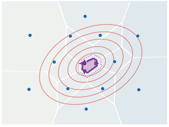
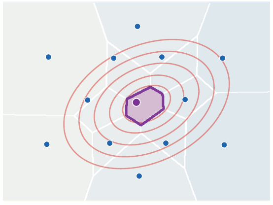
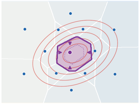
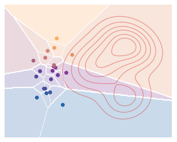
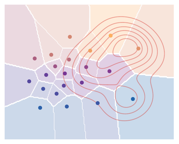
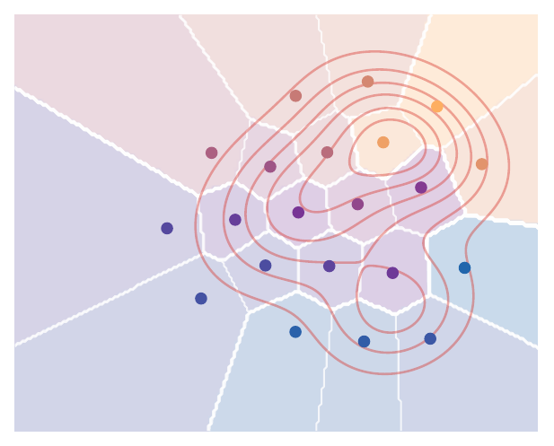
Live panel: Lloyd iterations
The iterations alternate cell assignment and centroid update.
Lloyd iterations
Lloyd descent is simple and robust, but it is nonconvex and can converge to local minima.
Quantization on the line
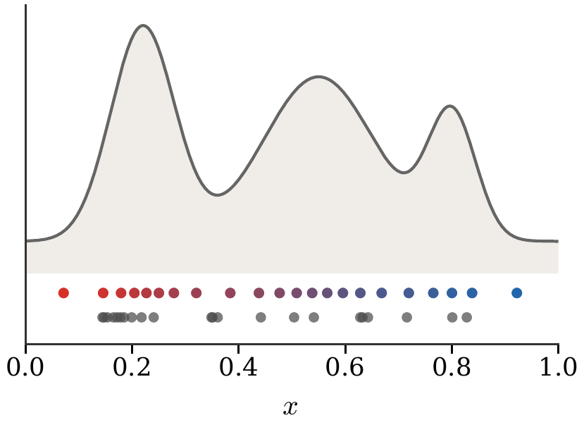
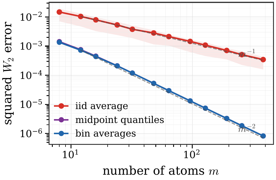
In one dimension, quantiles give explicit optimal placements for equal masses. This is much better than random sampling for W_2 approximation. For \alpha with quantile \textcolor{#c7372f}{F_\alpha^{-1}},
\textcolor{#226db4}{y_j}=\textcolor{#c7372f}{F_\alpha^{-1}}\!\left(\frac{j-\frac12}{m}\right)
is the canonical equal-mass placement.
Live panel: quantization rates
Optimal quantiles and random samples have visibly different convergence behavior.
Relaxed Lloyd flow
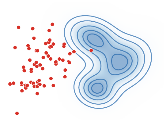
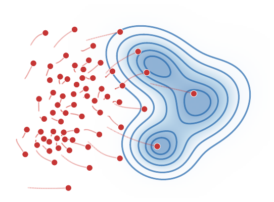
A slowed-down Lloyd update can be viewed as a continuous-time descent on the quantization energy in configuration space. For small relaxation parameter \eta,
\textcolor{#226db4}{y_j^{k+1}}=(1-\eta)\textcolor{#226db4}{y_j^k}+\eta\,\operatorname{centroid}(V_j(\textcolor{#226db4}{Y^k})).
Sites move toward a quantized representation of the target density.
Energy decay
The energy need not be globally convex, but standard Lloyd updates decrease it at each alternating minimization step.
Roadmap: links to learning
1. Duality
2. Wasserstein-1 and IPMs
3. Semi-discrete OT
4. Quantization
5. Learning links
Dual potentials as discriminators
The W_1 dual is the mathematical core of Wasserstein GANs, while other IPMs replace the Lipschitz ball by another function class.
TV
bounded witnesses
Wasserstein-1
Lipschitz witnesses
MMD
RKHS witnesses
Semi-discrete maps in applications
Semi-discrete OT appears when a continuous distribution is represented by a finite set of atoms:
- mesh generation and remeshing,
- color and texture processing,
- sampling and quantization,
- clustering with geometric costs,
- scalable approximations of continuous OT.
The computational object is a partition, not a dense coupling.
Linearized OT preview
Dual and semi-discrete ideas also feed linearized OT: fix a reference measure and embed nearby measures by displacement fields.
Live panel: linearized optimal transport
Linear OT turns transport maps into Euclidean coordinates for downstream analysis.
Summary
What this deck establishes. Duality turns transport into potentials. For W_1, these are Lipschitz witnesses. In the semi-discrete quadratic case, they are Laguerre weights defining a power diagram. Quantization and Lloyd algorithms reuse this geometry.
Dualitycertificates and gradients
 Wasserstein-1Lipschitz witnesses
 Laguerrecells and quantization