A centered Gaussian can be transformed into three Gaussian clouds in many ways. Two particularly interesting constructions are the deterministic diffusion map, obtained by reversing a score-based probability-flow ODE, and the optimal transport map, which minimizes the total squared displacement.
Both produce the same target distribution in the continuous model. But matching distributions does not mean matching individual particles. Coloring each particle by its destination makes this distinction visible.
The experiment: one Gaussian, three modes
In the plane, let
\[\begin{aligned} \mu&=\mathcal N(0,I_2),\\ \nu_\sigma&=\sum_{j=1}^{3}w_j\,\mathcal N(m_j,\sigma^2 I_2),\\ &\qquad \sum_jw_j=1. \end{aligned}\]The interactive example uses weights \((0.3,0.4,0.3)\) and means \(m_1=(-3,-2.3)\), \(m_2=(0,2)\), \(m_3=(5,-0.3)\). Positive \(\sigma\) gives three genuine Gaussian components; at \(\sigma=0\) the target becomes \(\sum_jw_j\delta_{m_j}\), the three-Dirac configuration of the reference sketch.
One Gaussian, three destinations, two maps
Diffusion Deterministic score ODE
Optimal transport Optimal matching of the same endpoints
A · blueB · cyanC · brown
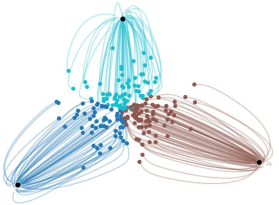
Reference sketch. Enable JavaScript for the interactive diffusion and optimal-transport comparison.
The two panels share their source points, target points, and spatial scale. Blue, cyan, and brown encode the destination, consistently in both panels. A particle can therefore change color between the two maps if it is assigned to a different mode. “Highlight mode changes” makes these particles stand out.
For overlapping Gaussians, color means the most probable component given the endpoint—not an intrinsic, uniquely recoverable latent label. In the Dirac limit, it is exactly the identity of the destination atom.
Diffusion: reverse a deterministic probability flow
Start with the target distribution and apply the Ornstein–Uhlenbeck noising process
\[\mathrm dY_t=-Y_t\,\mathrm dt+\sqrt{2}\,\mathrm dB_t, \qquad Y_0\sim\nu_\sigma.\]Its density \(p_t\) tends to the centered standard Gaussian. More explicitly,
\[\begin{aligned} p_t&=\sum_{j=1}^3w_j\, \mathcal N\!\left(e^{-t}m_j,a_t^2I_2\right),\\ a_t^2&=1-e^{-2t}+\sigma^2e^{-2t}. \end{aligned}\]Here and below, the same notation denotes a Gaussian law or its density. The score is \(\nabla\log p_t(x)\). The Fokker–Planck equation can be written as a continuity equation:
\[\begin{aligned} \partial_t p_t &=\Delta p_t+\nabla\cdot(xp_t)\\ &=-\nabla\cdot(p_t v_t),\\ v_t(x)&=-x-\nabla\log p_t(x). \end{aligned}\]Consequently, the deterministic ODE \(\dot x_t=v_t(x_t)\) has the same one-time marginal densities as the noising SDE. This is the probability-flow ODE, as used in Song et al., Score-Based Generative Modeling through Stochastic Differential Equations.
To generate data, integrate this ODE backward, from the Gaussian end toward the mixture. There is no injected noise along a trajectory: once the initial Gaussian point is fixed, the output is fixed.
An important factor-of-two warning: simply deleting the Brownian term from the reverse SDE does not give this ODE. For the normalization above, the forward-time probability-flow drift is \(-x-\nabla\log p_t\), whereas the reverse-SDE drift, expressed in decreasing forward time, is \(-x-2\nabla\log p_t\).
A map starting from an exact Gaussian
The OU process reaches its Gaussian equilibrium only as \(t\to\infty\). To avoid pretending that a finite noising time is exactly Gaussian, set \(r=e^{-t}\) and run \(r\) from \(0\) to \(1\). Write
\[\begin{aligned} q_r&=\sum_j w_j\mathcal N(rm_j,b_r^2I_2),\\ b_r^2&=1-r^2+\sigma^2r^2. \end{aligned}\]Then \(q_0=\mu\) and \(q_1=\nu_\sigma\) exactly. Define the generating flow by
\[\begin{aligned} \frac{\mathrm d}{\mathrm dr}\Phi_r(x) &=u_r(\Phi_r(x)),\\ \Phi_0(x)&=x,\\ u_r(z)&=\frac{z+\nabla\log q_r(z)}{r}. \end{aligned}\]The apparent singularity at \(r=0\) is removable. If
\[\begin{aligned} \pi_j(r,z) &=\frac{w_j\exp\!\left(-\frac{\|z-rm_j\|^2}{2b_r^2}\right)} {\sum_k w_k\exp\!\left(-\frac{\|z-rm_k\|^2}{2b_r^2}\right)},\\ \bar m_r(z)&=\sum_j\pi_j(r,z)m_j, \end{aligned}\]then the score and velocity are explicitly
\[\begin{aligned} \nabla\log q_r(z)&=\frac{r\bar m_r(z)-z}{b_r^2},\\ u_r(z)&=\frac{r(\sigma^2-1)z+\bar m_r(z)}{b_r^2}. \end{aligned}\]In particular, \(u_0(z)=\sum_jw_jm_j\). For \(\sigma>0\) this is a smooth flow through both endpoints. Its associated diffusion map is
\[\boxed{T_{\mathrm{diff}}=\Phi_1, \qquad (T_{\mathrm{diff}})_\#\mu=\nu_\sigma.}\]The push-forward notation means that \(T_{\mathrm{diff}}(X)\) has law \(\nu_\sigma\) when \(X\) has law \(\mu\). At zero width, the final map is understood as the limiting assignment to the atoms; it is no longer an invertible smooth map.
Optimal transport: optimize the assignment
The quadratic Monge problem instead asks for
\[\boxed{ T_{\mathrm{OT}}\in \underset{T_\#\mu=\nu_\sigma}{\operatorname{argmin}} \int\|T(x)-x\|^2\,\mathrm d\mu(x). }\]Since the source is absolutely continuous, Brenier’s theorem gives a unique optimal map, up to \(\mu\)-null sets, of the form \(T_{\mathrm{OT}}=\nabla\varphi\) with \(\varphi\) convex.
Its displacement interpolation is
\[X_s^{\mathrm{OT}}(x) =(1-s)x+sT_{\mathrm{OT}}(x), \qquad 0\leq s\leq1.\]Every particle travels along a straight segment at constant speed. These trajectories describe a Wasserstein geodesic; their intermediate distributions generally differ from the noising marginals followed backward by diffusion.
In the Dirac limit, the optimal map sends each source point to one of the three means. Its assignment regions are Laguerre cells:
\[\begin{aligned} c_j(x)&=\|x-m_j\|^2-\lambda_j,\\ L_j&=\{x:\ c_j(x)\leq c_k(x)\ \ \forall k\},\\ T_{\mathrm{OT}}(x)&=m_j\quad\text{on }L_j,\\ \mu(L_j)&=w_j. \end{aligned}\]The offsets \(\lambda_j\) enforce the prescribed masses. Subtracting the two squared distances leaves an affine inequality, so the cells are convex polygons, possibly unbounded. They are not, in general, ordinary nearest-center Voronoi cells. See the semi-discrete OT chapter for this geometric viewpoint.
Curved paths versus different maps
Curved diffusion trajectories and straight OT trajectories are visually striking, but curvature alone does not prove that the endpoint maps differ. One could follow a curved route and still reach the optimal endpoint.
The stronger distinction is the assignment. Diffusion transports mass along a prescribed path of densities; OT chooses the coupling that minimizes endpoint displacement. Although the diffusion velocity is a gradient at each instant, composing its infinitesimal maps need not produce the gradient of a convex function. In several dimensions, the Hessians encountered along a trajectory need not commute.
The displayed costs compare the assignments themselves:
\[\int\|T_{\mathrm{OT}}(x)-x\|^2\,\mathrm d\mu(x) \leq \int\|T_{\mathrm{diff}}(x)-x\|^2\,\mathrm d\mu(x).\]There are special cases of equality—for example, transport between a standard Gaussian and a single isotropic Gaussian. The point is not that diffusion can never be optimal, but that its construction does not impose optimality.
What the numerical figure computes
The source is a deterministic, equal-weight cloud of \(240\) points approximating \(\mathcal N(0,I_2)\). The left panel integrates the analytic mixture-score ODE with fourth-order Runge–Kutta; no score estimation or neural network is involved.
For comfortable playback, progress \(s\) uses the time change \(r=\sin(\pi s/2)\). This slows the final denoising stage without changing the trajectories or endpoint map. At \(\sigma=0\), integration stops just short of the singular endpoint and takes the limiting center assignment.
Let \(x_i\) be the source points and \(y_i\) their numerical diffusion endpoints. The right panel solves the unregularized finite assignment problem
\[\pi^\star\in\underset{\pi\in S_{240}}{\operatorname{argmin}} \sum_i\|x_i-y_{\pi(i)}\|^2\]using the Hungarian algorithm, and draws the straight segments \(x_i\to y_{\pi^\star(i)}\). It is exact OT between these two empirical measures, not a closed-form evaluation of the continuous Brenier map.
Reusing the same endpoints ensures that both panels have exactly the same empirical target, so the reported mean squared costs are directly comparable. The identity matching is feasible, hence the optimal-assignment cost cannot exceed the diffusion cost. In the Dirac limit, both panels also have identical counts at each atom; those finite-sample proportions approximate the prescribed weights.
Same Gaussian source, same target measure—but a different rule for deciding who goes where.