A positive Markov matrix repeatedly mixes probability vectors until they approach a single stationary distribution. Sinkhorn’s algorithm has a similar visual story: repeated application of a nonlinear map brings positive scaling vectors toward a distinguished ray.
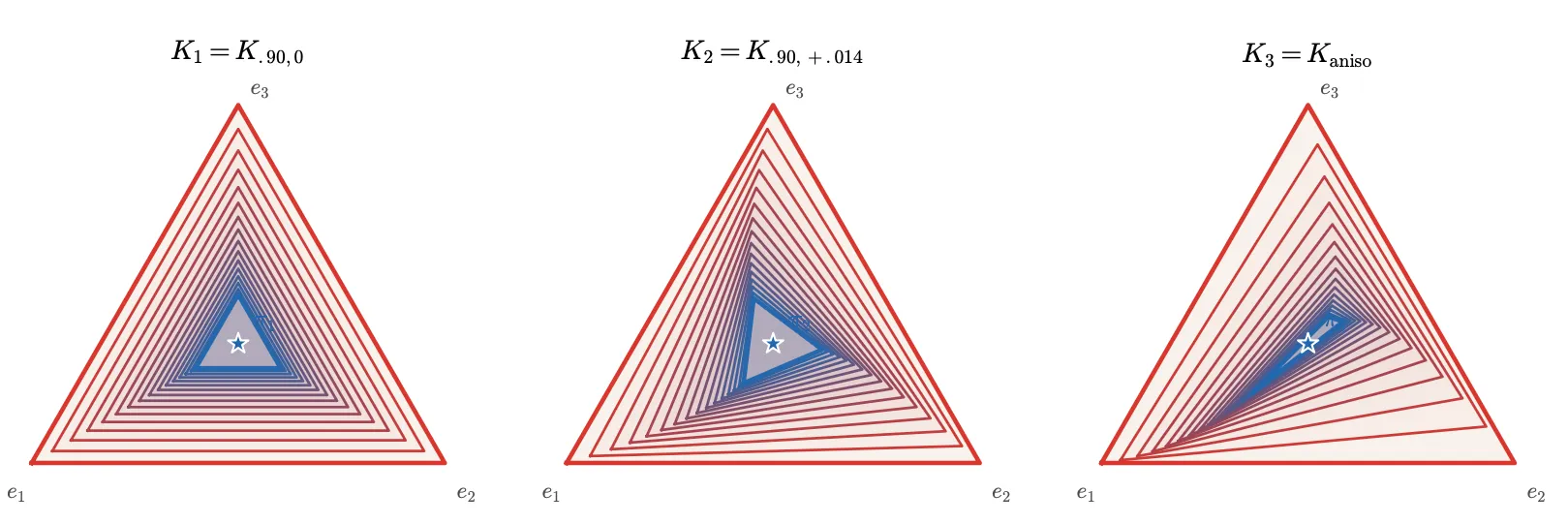
The analogy is particularly striking on the simplex of probability vectors with three entries — a triangle. Linear mixing shrinks straight-sided triangles; Sinkhorn bends them as it contracts. The appropriate geometry for the nonlinear picture is projective.
The linear picture
Let \(P\) be a strictly positive, column-stochastic matrix:
\[P_{ij}>0,\qquad \sum_i P_{ij}=1.\]It maps the simplex \(\Delta=\{p\geq0:\sum_i p_i=1\}\) into itself. Perron–Frobenius theory gives a unique stationary probability vector \(\pi>0\), and
\[p^{(k+1)}=Pp^{(k)},\qquad p^{(k)}\longrightarrow\pi.\]Strict positivity is important here: an arbitrary stochastic matrix can have several stationary distributions or periodic iterates.
The nonlinear picture
For strictly positive probability vectors \(a,b\) and a cost matrix \(C\), let \(K_{ij}=e^{-C_{ij}/\varepsilon}>0\). Entropically regularized optimal transport seeks
\[\min_{\substack{\Gamma\geq0\\\Gamma\mathbf1=a,\ \Gamma^\top\mathbf1=b}} \ \langle C,\Gamma\rangle +\varepsilon\sum_{ij}\Gamma_{ij}(\log\Gamma_{ij}-1).\]Its solution has the form \(\Gamma=\operatorname{diag}(u)K\operatorname{diag}(v)\). Alternately enforcing the two marginals gives
\[u=\frac{a}{Kv}, \qquad v_{\mathrm{new}}=\frac{b}{K^\top u},\]where division is componentwise. A complete iteration is therefore the nonlinear, positively homogeneous map
\[T(v)=\frac{b}{K^\top\!\left(a/(Kv)\right)}.\]The factors are only defined up to \(u\mapsto c^{-1}u\), \(v\mapsto cv\). To draw the iteration on a simplex, we remove this ambiguity by normalizing \(T(v)\) to sum to one.
Two ways to contract a simplex
Red to blue: successive images of the triangle. Thick blue boundary: the current image. Dark outlined dot: the limiting fixed point. The Markov matrix stays fixed as ε changes.
Enable JavaScript to use this figure’s animation and sliders. The equations and explanation remain available in the article.
The lower panel displays scaling vectors, not transport plans or transported probability distributions. At each step, the displayed marginal residual is computed from the corresponding matrix \(\Gamma\); it measures how far the current scaling is from satisfying both constraints.
To make the curved triangle images visible over many iterations, the example uses equal marginals \(a=b=(1/3,1/3,1/3)\) and a cost of zero on the diagonal and one off the diagonal. Thus
\[K= \begin{pmatrix} 1&\rho&\rho\\ \rho&1&\rho\\ \rho&\rho&1 \end{pmatrix}, \qquad \rho=e^{-1/\varepsilon}.\]At the default \(\varepsilon=0.22\), this kernel is close to the identity, so the contraction is gradual. Each boundary is obtained by applying the full nonlinear update to densely sampled points along all three edges. The map extends to the closed simplex because \(K\) is strictly positive. Step advances exactly one iteration; the playback-speed control changes only how long each iterate is shown.
Why “nonlinear Perron–Frobenius”?
For positive vectors, Hilbert’s projective distance is
\[d_{\mathrm H}(x,y) =\log\max_i\frac{x_i}{y_i} -\log\min_i\frac{x_i}{y_i}.\]It ignores an overall scale. Multiplication by a fixed positive vector and componentwise inversion preserve this distance, while a strictly positive matrix contracts it. Composing these operations explains the contraction of Sinkhorn’s map and convergence to its unique fixed ray.
This is not a claim that every visible Euclidean distance decreases at every step: the contraction is in a different geometry. Also, convergence solves the regularized transport problem; it approximates unregularized optimal transport as the regularization tends to zero.
For the scaling formulation and its projective geometry, see the computational optimal transport book with Marco Cuturi.