Take two positive numbers. Replace them simultaneously by their arithmetic and geometric means, then repeat. The numbers rapidly approach one another: their common limit is Gauss’s arithmetic–geometric mean. This simple algorithm connects averaging, dynamical systems, and elliptic integrals [1].
There are two different ways to generalize it. We can change coordinates before taking an arithmetic mean, or we can iterate two different averaging rules. The first construction gives quasi-arithmetic means; the second is called Gauss composition. Do these two constructions lead to the same family? Not in general—and there is an exact answer to when they do.
Three familiar means
For \(x,y>0\), the arithmetic, geometric, and harmonic means are
\[A(x,y)=\frac{x+y}{2},\qquad G(x,y)=\sqrt{xy},\qquad H(x,y)=\frac{2xy}{x+y}.\]All lie between their inputs, and
\[\min(x,y)\le H(x,y)\le G(x,y)\le A(x,y)\le\max(x,y).\]A short proof is \(A-G=(\sqrt x-\sqrt y)^2/2\ge0\), followed by \(H=G^2/A\le G\). The inequalities are strict between distinct means when \(x\ne y\).
Change coordinates: quasi-arithmetic means
Let \(I\subset\mathbb R\) be a nonempty open interval and \(f:I\to\mathbb R\) be continuous and strictly monotone. The function \(f\) is a generator, not itself a mean. Define
\[m_f(x,y)=f^{-1}\!\left(\frac{f(x)+f(y)}2\right), \qquad x,y\in I.\]This is a quasi-arithmetic mean, also called a Kolmogorov–Nagumo mean [2], [3]. Average in the \(f\)-coordinate, then come back. Continuity ensures that \(f(I)\) is an interval, so the inverse is defined at the midpoint. Strict monotonicity alone, without continuity, would not suffice.
The choices \(f(t)=t,\log t,1/t\) give \(A,G,H\), respectively. Decreasing generators are allowed. Every \(m_f\) is continuous, symmetric, strictly increasing in each argument, and strictly between distinct inputs. Moreover,
\[m_{af+b}=m_f\qquad(a\ne0).\]Only the coordinate system up to an affine change matters. Conversely, \(m_f=m_g\) implies \(g=af+b\): the continuous function \(g\circ f^{-1}\) preserves midpoints and is therefore affine.
Proposition 1 (compare generators by convexity). After choosing increasing generators,
\[m_f\le m_g\quad\Longleftrightarrow\quad g\circ f^{-1}\text{ is convex on }f(I).\]Proof: Jensen’s midpoint inequality in the right coordinate
Set \(u=f(x),v=f(y)\). Applying the increasing function \(g\) to the mean inequality gives
\[(g\circ f^{-1})\!\left(\frac{u+v}{2}\right) \le\frac{(g\circ f^{-1})(u)+(g\circ f^{-1})(v)}2.\]This is midpoint convexity; for a continuous function it is equivalent to convexity. The same calculation proves the converse. A decreasing generator can first be replaced by its negative, without changing its mean. \(\square\)
A useful one-parameter family is obtained from
\[f_p(t)=\begin{cases}(t^p-1)/p,&p\ne0,\\ \log t,&p=0.\end{cases}\]All these generators are increasing on \((0,\infty)\). Their power means are
\[P_p(x,y)=m_{f_p}(x,y) =\begin{cases}\bigl((x^p+y^p)/2\bigr)^{1/p},&p\ne0,\\ \sqrt{xy},&p=0.\end{cases}\]Thus \(P_{-1}=H,P_0=G,P_1=A\), and \(P_p\le P_q\) when \(p\le q\). For example, Proposition 1 proves this because \((f_q\circ f_p^{-1})'(f_p(t))=t^{q-p}\) is nondecreasing. The logarithmic case is included.
Iterate two means: Gauss composition
Given two generators \(f,g\), initialize \((x_0,y_0)=(x,y)\in I^2\) and iterate
\[x_{n+1}=m_f(x_n,y_n),\qquad y_{n+1}=m_g(x_n,y_n).\]Both updates use the old pair. Neither sequence needs to be monotone by itself: the two means can exchange their ordering. The correct objects to track are the lower and upper endpoints
\[a_n=\min(x_n,y_n),\qquad b_n=\max(x_n,y_n).\]Theorem 1 (existence, bounds, and uniqueness). Both sequences converge to a common limit \(M_{f,g}(x,y)\), called their Gauss composition. For every \(n\),
\[a_n\le a_{n+1}\le M_{f,g}(x,y) \le b_{n+1}\le b_n,\qquad b_n-a_n\longrightarrow0.\]The limit is a continuous, symmetric mean, nondecreasing in each argument and strictly between distinct inputs. It is the unique mean satisfying
\[M_{f,g}\bigl(m_f(x,y),m_g(x,y)\bigr)=M_{f,g}(x,y).\]Proof: nested intervals, not a contraction constant
Existence. Each new coordinate lies in the old interval, so \(a_n\uparrow a\) and \(b_n\downarrow b\). Symmetry of the two means gives
\[a_{n+1}=\min\{m_f(a_n,b_n),m_g(a_n,b_n)\}.\]If \(a<b\), continuity and strict internality imply
\[a=\min\{m_f(a,b),m_g(a,b)\}>a,\]a contradiction. Thus \(a=b\), squeezing both coordinates to the same limit. The first new interval already lies strictly inside the original one when \(x\ne y\).
Continuity and monotonicity. Each \(a_n,b_n\) is a continuous function of the initial pair. Their common limit is both a supremum of continuous lower bounds and an infimum of continuous upper bounds, hence continuous. Each coordinate of the iteration is nondecreasing in the initial inputs, so the limit is too. Symmetry also passes to the limit. On compact subsets, the endpoint convergence is uniform by Dini’s theorem.
Uniqueness. Dropping the first iterate leaves the limit unchanged, proving invariance. If another internal function \(K\) satisfies the same equation, then
\[K(x,y)=K(x_n,y_n)\in[a_n,b_n]\]for every \(n\), so \(K(x,y)=M_{f,g}(x,y)\). This last argument does not even require continuity of \(K\). \(\square\)
The convergence, continuity, internality, and uniqueness argument works for any two continuous symmetric strict means, not just quasi-arithmetic ones. Monotonicity of the limit additionally uses monotonicity of the input means. Without strictness, convergence can fail: iterating \((\min,\max)\) leaves a distinct pair unchanged.
The first-step sandwich is especially useful:
\[\min(m_f,m_g)\le M_{f,g}\le\max(m_f,m_g).\]Sharper bounds cost only more iterations. The midpoint of \([a_n,b_n]\) approximates the limit with error at most \((b_n-a_n)/2\) in exact arithmetic. Swapping \(f,g\) changes nothing. If both input means are homogeneous, so is the limit. More generally, changing coordinates conjugates the entire iteration: a continuous strictly monotone \(r\) sends \(M_{f,g}\) to the composition generated by \(f\circ r^{-1},g\circ r^{-1}\).
Arithmetic–geometric versus arithmetic–harmonic
The classical choice \(m_f=A,m_g=G\) gives
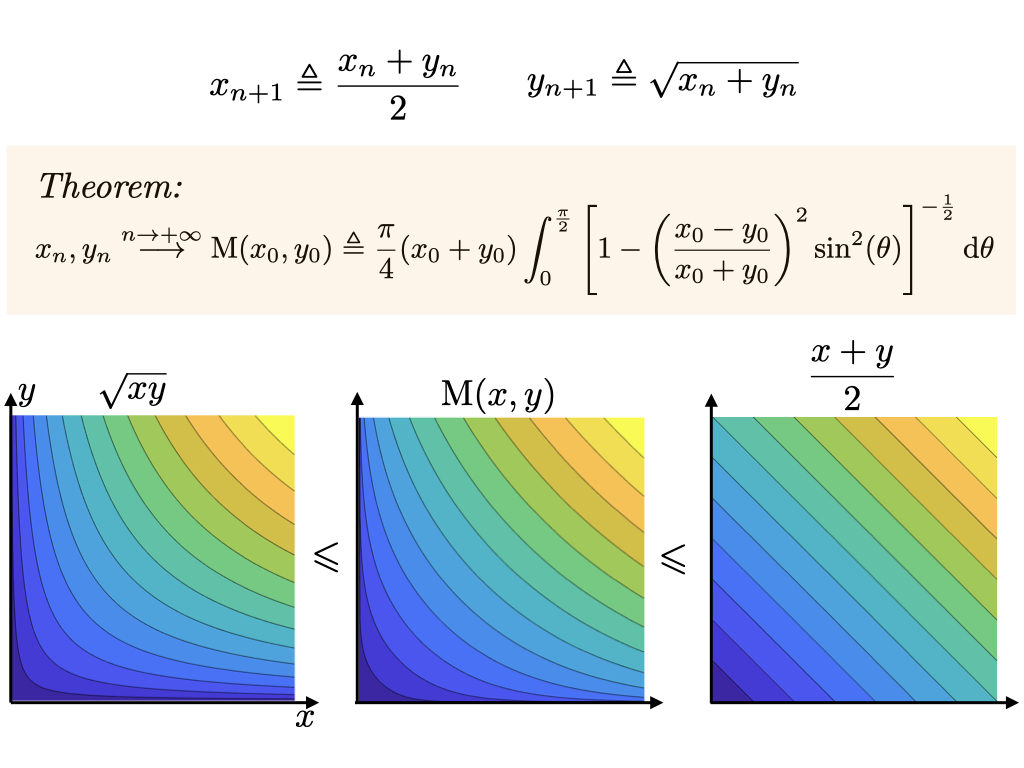
\[G(x,y)\le\operatorname{AGM}(x,y)\le A(x,y).\]Its speed is visible from one identity:
\[A(x,y)-G(x,y) =\frac{(x-y)^2}{2(\sqrt x+\sqrt y)^2}.\]Once the numbers are close and bounded away from zero, the new gap is proportional to the square of the old gap. This is quadratic convergence. The same AGM computes complete elliptic integrals, for instance
\[K(k)=\int_0^{\pi/2}\frac{d\theta}{\sqrt{1-k^2\sin^2\theta}} =\frac{\pi}{2\operatorname{AGM}(1,\sqrt{1-k^2})},\qquad 0\le k<1,\]a classical connection recorded in [1].
For the pair \(A,H\), there is an even simpler answer.
Proposition 2 (arithmetic–harmonic iteration gives the geometric mean).
\[M_{\mathrm{id},\,1/\mathrm{id}}(x,y)=\sqrt{xy}.\]Proof: the product is conserved
The identity \(A(x,y)H(x,y)=xy\) gives \(x_ny_n=xy\) at every step. At the common positive limit \(L\), this becomes \(L^2=xy\). Thus \(L=\sqrt{xy}\). Equivalently, \(G(A,H)=G\), and uniqueness in Theorem 1 identifies the invariant mean. \(\square\)
This also holds for opposite power means: \(P_p(x,y)P_{-p}(x,y)=xy\), hence their Gauss composition is \(G\). At the other extreme, composing a mean with itself just returns that mean after one step.
When is the limit another quasi-arithmetic mean?
The natural question is whether \(M_{f,g}=m_h\) for some generator \(h\). The answer is unexpectedly rigid. A fractional-linear, or Möbius, function is \(u\mapsto(au+b)/(cu+d)\), with \(ad-bc\ne0\) and no pole on the interval being used.


Theorem 2 (Daróczy–Páles, in fractional-linear form). Let \(f,g:I\to\mathbb R\) be continuous strictly monotone generators on an open interval. Then \(M_{f,g}\) is quasi-arithmetic if and only if
\[g(x)=\frac{af(x)+b}{cf(x)+d},\qquad ad-bc\ne0,\qquad cf(x)+d\ne0\quad(x\in I).\]If \(c=0\), the two input means coincide and \(M_{f,g}=m_f\). If \(c\ne0\), then
\[M_{f,g}=m_h,\qquad h(x)=\log|cf(x)+d|.\]This is an equivalent formulation of their complete solution of the Matkowski–Sutő problem [4, Theorems 4.12 and 4.14]. No differentiability is assumed.
Proof: the explicit construction and the rigidity step
Sufficiency is elementary. If \(c=0\), \(g\) is an affine change of \(f\). Otherwise \(F=|cf+d|>0\) is itself a continuous strictly monotone generator. Since its sign before taking the absolute value is constant, \(m_F=m_f\), and \(g\) is an affine change of \(1/F\). Consequently, in the \(F\)-coordinate, the iteration is precisely
\[F(x_{n+1})=A(F(x_n),F(y_n)),\qquad F(y_{n+1})=H(F(x_n),F(y_n)).\]Proposition 2 shows that its limit satisfies \(F(M_{f,g}(x,y))=\sqrt{F(x)F(y)}\). Taking logarithms gives \(M_{f,g}=m_{\log F}\).
Necessity reduces to complementary means. Suppose \(M_{f,g}=m_h\). Set \(J=h(I)\), \(\varphi=f\circ h^{-1}\), and \(\psi=g\circ h^{-1}\). The invariance equation, after applying \(h\), becomes
\[m_\varphi(u,v)+m_\psi(u,v)=u+v,\qquad u,v\in J.\]The required rigidity result says that, up to independent nonconstant affine changes, \(\varphi,\psi\) are either both the identity, or \(e^{pu},e^{-pu}\) for one \(p\ne0\). In the first case \(g\) is affine in \(f\). In the second,
\[f=\alpha e^{ph}+\beta,\qquad g=\gamma e^{-ph}+\delta,\qquad\alpha\gamma\ne0,\]so \((f-\beta)(g-\delta)=\alpha\gamma\), which is exactly a nonaffine fractional-linear relation. This finishes the reduction. \(\square\)
A self-contained proof of rigidity for smooth generators
Assume here that \(\varphi,\psi\in C^4(J)\) have nowhere-zero derivatives. Put \(P=\varphi''/\varphi'\) and \(Q=\psi''/\psi'\). Taylor expansion around the diagonal gives
\[m_\varphi(t+s,t-s) =t+\frac{P(t)}2s^2 +\frac{P''+3PP'-2P^3}{24}(t)s^4+o(s^4).\]Check the expansion by solving for the midpoint
Write the mean as \(t+a s^2+b s^4+o(s^4)\). In the identity defining it, the right side is \(\varphi(t)+\varphi''(t)s^2/2+\varphi^{(4)}(t)s^4/24+o(s^4)\). Expanding the left side gives
\[a=\frac{\varphi''}{2\varphi'}=\frac P2,\qquad b=\frac{\varphi^{(4)}}{24\varphi'}-\frac{P^3}{8}.\]Finally \(\varphi^{(4)}/\varphi'=P''+3PP'+P^3\), yielding the displayed formula. \(\square\)
The complementary-mean identity forces the \(s^2\) coefficients to cancel, so \(Q=-P\). The sum of the \(s^4\) coefficients is then \(PP'/4\), hence \(PP'=0\). Thus \((P^2)'=0\). Continuity on the connected interval makes \(P\) a single constant \(p\). Solving
\[\varphi''=p\varphi',\qquad\psi''=-p\psi'\]gives the affine or opposite-exponential alternatives. Conversely, for \(p\ne0\), direct algebra gives
\[\frac1p\log\frac{e^{pu}+e^{pv}}2 -\frac1p\log\frac{e^{-pu}+e^{-pv}}2=u+v.\]For \(p=0\), both means are arithmetic. This proves rigidity under the stated smoothness hypotheses. \(\square\)
What is needed for the full continuous theorem?
The Taylor proof does not establish the merely continuous case. Daróczy–Páles first obtain local \(C^1\) regularity with nonzero derivatives, solve the equation there, and propagate that solution across the interval [4, Theorems 4.11, 3.6, and 3.14]. Their argument uses real-analysis tools including almost-everywhere differentiability and Baire category. This non-elementary regularity-and-extension step is quoted here; the construction, reduction, and smooth rigidity proof above are self-contained. In particular, one must not differentiate \(h\) merely because the original \(f,g\) happen to be smooth.
The interpretation is simple: apart from composing a mean with itself, every quasi-arithmetic answer is a change of coordinates of arithmetic–harmonic iteration. But not every iteration has such an answer. In particular, the classical AGM is not quasi-arithmetic: its generators \(t\) and \(\log t\) are not related by a fractional-linear transformation.
Why the logarithm cannot be fractional-linear in the identity
The affine possibility is impossible since \((\log t)''\ne0\). A nonaffine possibility would imply \((t-\beta)(\log t-\delta)=k\) on an open positive interval. Differentiating twice would give \((t+\beta)/t^2=0\) throughout that interval, which is impossible. \(\square\)
Numerical experimentation
The first slider explores \(P_p(x,y)\), including harmonic, geometric, and arithmetic averaging. Together with the second slider it chooses the pair \(P_p,P_q\) whose Gauss composition is displayed alongside it. Select a point in a heatmap to follow the shrinking bracket; both coordinates are updated simultaneously. Try the arithmetic–geometric and arithmetic–harmonic presets, or \(p=q\), when the limit is reached after one step.
The plots evaluate actual power means and their numerical iterates, not a fitted approximation. Positive inputs avoid singularities at zero. The final bracket supplies an exact-arithmetic error bound; ordinary floating-point computations are not interval arithmetic. The panel distinguishes tolerance, roundoff, and an iteration cap. Its design is inspired by my arithmetic–geometric vignette and its companion notebook.
References
- NIST Digital Library of Mathematical Functions. §19.8(i), Gauss’s Arithmetic-Geometric Mean (AGM). Reference and formulas.
- Mitio Nagumo. Über eine Klasse der Mittelwerte. Japanese Journal of Mathematics 7, 71–79, 1930. Paper.
- Janusz Matkowski and Zsolt Páles. Characterization of generalized quasi-arithmetic means. Acta Scientiarum Mathematicarum (Szeged) 81, 447–456, 2015. Paper.
- Zoltán Daróczy and Zsolt Páles. Gauss-composition of means and the solution of the Matkowski–Sutô problem. Publicationes Mathematicae Debrecen 61(1–2), 157–218, 2002. Paper.