A discrepancy between probability distributions can be built in two quite different ways. We can compare their density ratio at each point. Or we can measure how far a convex functional lies above its tangent plane. The first construction comes from statistical information; the second comes from convex geometry and optimization.
Kullback–Leibler divergence belongs to both families. This is more than a convenient coincidence: under natural smoothness assumptions, it is the only common member, up to scale. A short proof reveals why entropy appears so often when probability models meet convex optimization.
The finite-alphabet characterization is Theorem 5 of Jiao, Courtade, No, Venkat, and Weissman [1]. The measure-level formulation below follows Proposition 8.34 of Optimal Transport for Machine Learners [2]. We start with the two definitions, because similar-looking quadratic formulas can disguise genuinely different geometries.

Imre Csiszár
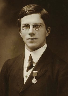
Ronald Fisher
First construction: compare density ratios
Let \(\alpha=p\,\omega\) and \(\beta=q\,\omega\) be probability measures with positive densities relative to a finite reference measure \(\omega\). For a convex function \(\phi:(0,\infty)\to\mathbb R\) satisfying \(\phi(1)=0\), define the \(\phi\)-divergence, also called an \(f\)-divergence, by
\[D_\phi(\alpha\mid\beta) =\int q(x)\phi\!\left(\frac{p(x)}{q(x)}\right)\,d\omega(x).\]This depends only on \(\alpha,\beta\), not on the choice of dominating measure. Jensen's inequality under \(\beta\) gives \(D_\phi\ge\phi(\int p\,d\omega)=0\). If \(\phi\) is strictly convex, equality holds only for equal measures.
Three standard examples are
\[\begin{array}{c|c} \phi(r)&D_\phi(\alpha\mid\beta)\\ \hline r\log r-r+1 & \displaystyle\int p\log(p/q)\,d\omega\\[3pt] (r-1)^2/2 & \displaystyle\frac12\int\frac{(p-q)^2}{q}\,d\omega\\[3pt] (\sqrt r-1)^2 & \displaystyle\int(\sqrt p-\sqrt q)^2\,d\omega . \end{array}\]These are KL, half the Pearson \(\chi^2\) divergence, and squared Hellinger distance with the displayed normalization. For probabilities, the linear terms in the KL generator integrate to zero. More generally, replacing \(\phi(r)\) by \(\phi(r)+a(r-1)\) leaves the divergence unchanged.
One family, several geometries
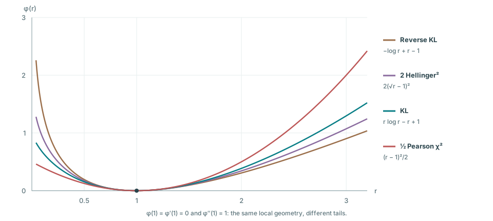
To compare shapes rather than arbitrary linear terms, normalize the generators by \(\phi(1)=\phi'(1)=0\). For the pictures, also fix \(\phi''(1)=1\). A convenient power-divergence family is [7]
\[\phi_\lambda(r)= \begin{cases} \displaystyle\frac{r^\lambda-1-\lambda(r-1)}{\lambda(\lambda-1)},&\lambda\notin\{0,1\},\\[5pt] -\log r+r-1,&\lambda=0,\\[2pt] r\log r-r+1,&\lambda=1. \end{cases}\]The cases \(0\) and \(1\) are the continuous limits in the parameter. Since \(\phi_\lambda''(r)=r^{\lambda-2}>0\), every member is strictly convex. For \(\lambda=0,\frac12,1,2\), the corresponding divergences are reverse KL, twice the squared Hellinger distance displayed above, KL, and half Pearson \(\chi^2\). Our parameter is one larger than the parameter in Cressie–Read’s original convention.
Definition at zero densities and for singular measures
Write the Lebesgue decomposition \(\alpha=f\,\beta+\alpha^\perp\), with \(\alpha^\perp\) singular relative to \(\beta\). The lower-semicontinuous extension is
\[D_\phi(\alpha\mid\beta) =\int\phi(f)\,d\beta+\phi'_\infty\,\alpha^\perp(E), \qquad \phi'_\infty=\lim_{r\to\infty}\frac{\phi(r)}r.\]At \(f=0\), use \(\phi(0)=\lim_{r\downarrow0}\phi(r)\), possibly infinite, and use \(0\cdot\infty=0\) for a vanishing singular mass. For KL, \(\phi'_\infty=+\infty\): any nonzero part of \(\alpha\) singular with respect to \(\beta\) gives infinite divergence, even if their topological supports overlap. The smooth theorem below stays inside strictly positive bounded densities, where no such convention is needed.
Second construction: subtract a tangent plane
Let \(\Phi\) be a differentiable convex functional on a convex set of densities. Its Bregman divergence is
\[B_\Phi(\alpha\mid\beta) =\Phi(\alpha)-\Phi(\beta) -\int\delta\Phi(\beta)\,d(\alpha-\beta).\]The first variation \(\delta\Phi(\beta)\) describes the tangent plane at \(\beta\); convexity makes the remainder nonnegative. On probability measures, the first variation is defined only up to an additive constant, which disappears because \(\alpha-\beta\) has total mass zero. This construction goes back to Bregman [3].
For a separable functional \(\Phi(p\,\omega)=\int F(p)\,d\omega\),
\[B_\Phi(\alpha\mid\beta) =\int\bigl[F(p)-F(q)-F'(q)(p-q)\bigr]\,d\omega.\]Choosing \(F(r)=r^2/2\) gives \(\frac12\int(p-q)^2\,d\omega\). Notice the missing factor \(1/q\): this is squared \(L^2(\omega)\) error, not Pearson divergence. It changes if the reference measure changes while the formula for \(F\) is held fixed.
Choosing \(F(r)=r\log r-r\) instead gives
\[F(p)-F(q)-F'(q)(p-q) =p\log(p/q)-p+q.\]After integration over probabilities, this is KL. This is the first meeting of the two constructions, historically introduced in information theory by Kullback and Leibler [4].
Bregman generators need not be pointwise integrals. For a bounded feature map \(\psi:E\to\mathbb R^k\), the nonlocal functional
\[\Phi(\alpha)=\frac12\left|\int\psi\,d\alpha\right|^2\]has divergence \(\frac12|\int\psi\,d\alpha-\int\psi\,d\beta|^2\). It can vanish for different measures with the same features. “Divergence” therefore does not automatically mean a metric, or even a discrepancy separating every pair of laws.
A short rigidity theorem
For a precise domain, normalize the finite reference measure so that \(\omega(E)=1\), and assume it has a measurable set \(A\) with \(0<\omega(A)<1\). Let \(\mathcal D\) be all probability densities bounded above and bounded away from zero; the bounds may depend on the density.
Theorem 1 (the smooth intersection is KL). Suppose \(\phi\in C^2(0,\infty)\) is convex with \(\phi(1)=0\), and \(\Phi\) is convex and twice differentiable along bounded zero-mass density directions. If
\[B_\Phi(p\,\omega\mid q\,\omega) =D_\phi(p\,\omega\mid q\,\omega) \quad\text{for all }p,q\in\mathcal D,\]then, for some \(\kappa\ge0\),
\[B_\Phi=D_\phi=\kappa\,\mathrm{KL}.\]More precisely, \(\phi(r)=\kappa r\log r+a(r-1)\), and \(\Phi\) differs from \(\kappa\int p\log p\,d\omega\) by an affine functional on \(\mathcal D\).
Proof: the local Hessian determines the global Bregman divergence
Step 1: compare second derivatives at equal densities. Fix \(q\in\mathcal D\) and a bounded \(h\) with \(\int h\,d\omega=0\). For sufficiently small \(t\), \(q+th\in\mathcal D\). Differentiate the asserted equality twice at \(t=0\):
\[D^2\Phi(q)[h,h] =\phi''(1)\int\frac{h^2}{q}\,d\omega.\]Set \(\kappa=\phi''(1)\ge0\). The right-hand side is exactly the second derivative of \(\kappa\operatorname{Ent}(q)=\kappa\int q\log q\,d\omega\). Thus \(\Psi=\Phi-\kappa\operatorname{Ent}\) has zero second derivative along every segment in \(\mathcal D\).
Consequently \(\Psi\) is affine on each such segment, so its tangent-plane remainder is zero. Therefore \(B_\Phi=\kappa B_{\operatorname{Ent}}=\kappa\mathrm{KL}\) for all pairs—not just infinitesimally close pairs.
Step 2: recover the scalar generator. Put \(\psi(s)=\phi(s)-\kappa s\log s\). We now know that \(\int q\,\psi(p/q)\,d\omega=0\) for every pair.
Two-value lemma: a zero probability divergence is linear
Choose any \(0<x<1<y\), and set
\[w=\frac{y-1}{y-x},\qquad 1-w=\frac{1-x}{y-x}.\]Choose \(q\) constant on \(A\) and \(A^c\), with \(\beta(A)=w\). Set \(p=xq\) on \(A\) and \(p=yq\) on \(A^c\). Both are strictly positive bounded probability densities because \(wx+(1-w)y=1\). The zero divergence yields
\[(y-1)\psi(x)+(1-x)\psi(y)=0,\]hence \(\psi(x)/(x-1)=\psi(y)/(y-1)\). Varying \(x\) and \(y\) shows this ratio has the same constant value on both sides of one. Since \(\psi(1)=0\), \(\psi(s)=a(s-1)\) everywhere.
This proves the scalar formula and completes the characterization. \(\square\)
The two-point construction explains the minimal assumption on the reference space: it must distinguish at least two events. On a one-point probability space every divergence is zero, so no generator can be identified.
The theorem also allows nonseparable \(\Phi\). It does not assume in advance that the Bregman generator is an integral of a scalar function. Its Hessian is forced to be that of entropy simply by matching the density-ratio divergence at every base density.
Local agreement alone is much weaker. Every smooth \(\phi\)-divergence has, for a bounded zero-mass perturbation \(h\), the expansion
\[D_\phi((q+th)\omega\mid q\omega) =\frac{\phi''(1)t^2}{2} \int\frac{h^2}{q}\,d\omega+o(t^2).\]This common quadratic form is the Fisher information metric; it does not make Hellinger or Pearson divergence equal to KL. Rigidity comes from requiring one Bregman generator to realize the divergence for all pairs. Its Hessian at every base point then determines its tangent-plane remainders globally. If the divergence separates distinct laws, the scale in Theorem 1 must satisfy \(\kappa>0\); \(\kappa=0\) gives the identically zero divergence.
Why this matters for algorithms
The derivative of entropy is logarithmic. On a finite probability simplex, minimizing a linear cost regularized by KL gives an explicit multiplicative step:
\[\begin{aligned} p^\star&=\underset{p_i\ge0,\ \sum_i p_i=1}{\arg\min} \left\{\sum_i c_ip_i+\frac1\eta\mathrm{KL}(p\mid q)\right\},\\ p_i^\star&=\frac{q_i e^{-\eta c_i}} {\sum_jq_j e^{-\eta c_j}}, \qquad q_i>0,\quad\eta>0. \end{aligned}\]A Lagrange multiplier for total mass makes \(\log(p_i/q_i)+\eta c_i\) constant, which gives the formula. Entropy geometry turns an additive change in dual coordinates into multiplicative reweighting in probability coordinates.
The overlap theorem explains why KL simultaneously enjoys a density-ratio interpretation and a tangent-plane interpretation. It does not say that other divergences are inferior. Pearson, Hellinger, squared density error, and feature-mean errors encode different choices. What it rules out is freely exchanging their geometric formulas merely because all of them measure a discrepancy.
Numerical experimentation: a triangle of probabilities
Three nonnegative probabilities summing to one form a two-dimensional triangle inside \(\mathbb R^3\):
\[\Delta_3=\left\{q\in\mathbb R_+^3:\sum_{i=1}^3q_i=1\right\}.\]Here write \(q\) for the varying point and \(p\) for the target. The figure evaluates the same density-ratio construction
\[D_{\phi_\lambda}(q\mid p) =\sum_{i=1}^3p_i\phi_\lambda(q_i/p_i).\]Change \(\lambda\) to move between the four familiar examples, and click or drag in the triangle to move \(p\). The two target-coordinate sliders provide the same control without a pointer. Contours bend as the generator changes, even though all these divergences have the same second-order Fisher geometry at the target. This plot is not the Bregman divergence of \(\phi_\lambda\); only the KL member belongs to both families in the sense of Theorem 1.
Targets are projected to \(p_i\ge0.04\), while the plotted \(q\) ranges over the whole closed triangle. Reverse KL is infinite on its boundary. The fixed color scale saturates at four; finite contours use a triangular grid and omit cells with an infinite corner. Changing the plot resolution does not change the divergence definition.
References
- Jiantao Jiao, Thomas A. Courtade, Albert No, Kartik Venkat, and Tsachy Weissman. Information Measures: The Curious Case of the Binary Alphabet. IEEE Transactions on Information Theory 60(12), 7616–7626, 2014. Theorem 5.
- Gabriel Peyré. Optimal Transport for Machine Learners, Proposition 8.34, Definition 8.31, and Definition 7.16. Book manuscript.
- Lev M. Bregman. The Relaxation Method of Finding the Common Point of Convex Sets and Its Application to the Solution of Problems in Convex Programming. USSR Computational Mathematics and Mathematical Physics 7(3), 200–217, 1967.
- Solomon Kullback and Richard A. Leibler. On Information and Sufficiency. Annals of Mathematical Statistics 22(1), 79–86, 1951.
- Imre Csiszár. Information-type measures of difference of probability distributions and indirect observations. Studia Scientiarum Mathematicarum Hungarica 2, 299–318, 1967. Author’s publication list, item 13.
- Ronald A. Fisher. On the Mathematical Foundations of Theoretical Statistics. Philosophical Transactions of the Royal Society A 222, 309–368, 1922. Author archive.
- Noel Cressie and Timothy R. C. Read. Multinomial Goodness-of-Fit Tests. Journal of the Royal Statistical Society, Series B 46(3), 440–464, 1984.