A dataset is often better represented by a probability measure than by a vector. A point cloud may contain ten points or ten thousand; its ordering should not matter. A population in a mean field game has the same feature: what matters is the distribution of states, rather than a list of named individuals. This raises a basic approximation question: what are the analogues of polynomials when the input is a whole probability distribution?
The answer is pleasantly concrete. Start with expectations of continuous features, multiply a finite number of them, and take linear combinations. On a compact ground space, these expressions approximate every continuous functional of a probability measure, uniformly over all measures. The proof is a direct application of Stone–Weierstrass. It explains why averaging features can be a universal architecture, and why finite-particle interactions are useful coordinates for an infinite-dimensional space. This is also the subject of the “Measure-to-Vector Maps on Wasserstein Space” section of my book [1].
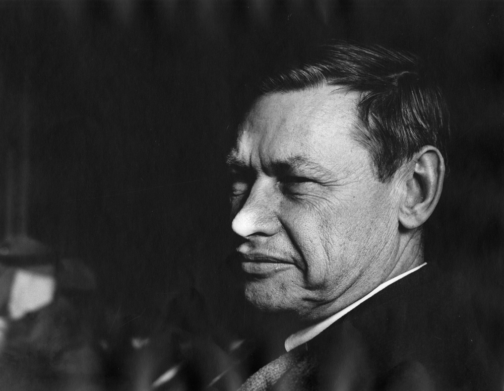
Marshall H. Stone
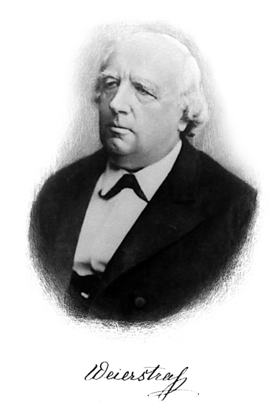
Karl Weierstrass
A compact space whose points are measures
Let \((K,d)\) be a nonempty compact metric space and let \(\mathcal P(K)\) be its Borel probability measures. Fix \(1\le p<\infty\). The Wasserstein distance is
\[ W_p(\mu,\nu)^p =\inf_{\pi\in\Pi(\mu,\nu)}\int_{K\times K}d(x,y)^p\,d\pi(x,y), \]where \(\Pi(\mu,\nu)\) contains the joint laws with marginals \(\mu\) and \(\nu\). Because \(K\) is compact, \(\mathcal P(K)\) is compact too, and convergence in \(W_p\) is equivalent to weak convergence: convergence of \(\int\phi\,d\mu\) for every \(\phi\in C(K)\). Thus all finite choices of \(p\) give the same continuous functionals here [1].
For a continuous feature \(\phi:K\to\mathbb R\), write
\[ m_\phi(\mu)=\int_K\phi(x)\,d\mu(x). \]This is a linear observable of the measure. Its dependence on the point \(x\) can be completely nonlinear: \(\phi\) could be a cosine, a bump, or a neural-network feature.
What is a polynomial of a measure?
A moment polynomial is a finite linear combination of products
\[ M(\mu)=\prod_{j=1}^{r}m_{\phi_j}(\mu). \]The empty product is \(1\). More generally, a continuous interaction kernel \(\Phi:K^r\to\mathbb R\) defines a Wasserstein polynomial of order at most \(r\):
\[ P_\Phi(\mu)=\int_{K^r}\Phi(x_1,\ldots,x_r)\,d\mu^{\otimes r}. \]Equivalently, draw independent \(X_1,\ldots,X_r\) with law \(\mu\), and take \(\mathbb E\Phi(X_1,\ldots,X_r)\). The order counts how many particles interact; it does not count powers of their spatial coordinates. Symmetrizing \(\Phi\) leaves \(P_\Phi\) unchanged. Lower-order terms can be included by adding dummy variables, since \(\mu(K)=1\).
Why call this a polynomial? Along a mixture \(\mu_t=(1-t)\mu+t\nu\), the value \(P_\Phi(\mu_t)\) is an ordinary polynomial in \(t\), of degree at most \(r\): simply expand the \(r\) factors of \(\mu_t^{\otimes r}\). This is a statement about mixing measures, not about moving their particles along a Wasserstein geodesic.
Every moment monomial is such an interaction, with \(\Phi(x_1,\ldots,x_r)=\prod_j\phi_j(x_j)\). A general continuous kernel need not be an exact finite sum of these separated products. However, Stone–Weierstrass on \(K^r\) approximates it by such sums; integration preserves the uniform error. The two classes therefore have the same uniform closure.
For example, on a compact subset of \(\mathbb R\), variance is an order-two polynomial:
\[ \operatorname{Var}(\mu) =m_{x^2}(\mu)-m_x(\mu)^2 =\frac12\iint(x-y)^2\,d\mu(x)d\mu(y). \]Likewise, \(\iint V(x,y)\,d\mu(x)d\mu(y)\) describes a pair interaction. By contrast, \(\mu\mapsto W_p(\mu,\nu)\), with a fixed target \(\nu\), is typically not itself a finite polynomial. It is continuous, so the next theorem still applies.
Universality in three observations
Theorem 1 (polynomial universality). For every continuous \(F:\mathcal P(K)\to\mathbb R\) and every \(\varepsilon>0\), there is a moment polynomial \(P\) such that
\[ \sup_{\mu\in\mathcal P(K)}|F(\mu)-P(\mu)|<\varepsilon. \]In particular, Wasserstein polynomials are uniformly dense. This classical argument appears explicitly in Cardaliaguet’s notes on mean field games, §5.3, Proposition 5.9 [2].
Proof: constants, products, and separation
Let \(\mathcal A\) be the moment polynomials. Every member is continuous. Constants belong to \(\mathcal A\), and multiplying two finite products gives another finite product; hence \(\mathcal A\) is a unital algebra.
If \(\mu\ne\nu\), some continuous \(\phi\) satisfies \(\int\phi\,d\mu\ne\int\phi\,d\nu\): continuous test functions determine Borel measures on a compact metric space. The order-one observables therefore already separate measures.
The real Stone–Weierstrass theorem [3], applied to the compact space \(\mathcal P(K)\), gives \(\overline{\mathcal A}=C(\mathcal P(K))\). \(\square\)
The crucial distinction is between one fixed finite list of moments and a list that may grow with the desired accuracy. Two distributions can have the same mean and variance. The theorem allows us to add the features needed to distinguish the distributions relevant to the target functional.
An explicit approximation: sample, evaluate, average
Stone–Weierstrass proves existence. There is also a natural construction. For independent samples \(X_i\sim\mu\), define the empirical measure and its averaged prediction:
\[ \widehat\mu_n=\frac1n\sum_{i=1}^n\delta_{X_i}, \qquad B_nF(\mu)=\mathbb E F(\widehat\mu_n). \]This is a Wasserstein polynomial of order at most \(n\), with symmetric kernel \(\Phi_n(x_1,\ldots,x_n)=F(n^{-1}\sum_i\delta_{x_i})\). The kernel is continuous: pairing corresponding points bounds the Wasserstein distance between their empirical measures by their largest displacement. These are Bernstein–Schnabl operators [4]. For \(K=\{0,1\}\), writing \(\mu_t=(1-t)\delta_0+t\delta_1\), the formula reduces to the ordinary Bernstein polynomial
\[ B_nF(\mu_t)=\sum_{k=0}^{n}F(\mu_{k/n}) \binom nk t^k(1-t)^{n-k}. \]Theorem 2 (uniform particle approximation). For every \(F\in C(\mathcal P(K))\),
\[ \sup_{\mu\in\mathcal P(K)}|B_nF(\mu)-F(\mu)|\longrightarrow0. \]The uniformity is important: the same number of particles works for all input measures. Pointwise convergence of empirical measures alone would not prove this stronger statement.
Proof: repeated sample indices are the only error on monomials
Lemma 1. If \(M=\prod_{j=1}^r m_{\phi_j}\), with \(r\ge1\) and \(n\ge r\), then
\[ \|B_nM-M\|_\infty \le\frac{r(r-1)}n\prod_{j=1}^r\|\phi_j\|_\infty. \]Proof of Lemma 1: expand the sample averages
For \(r=1\), equality is exact. Otherwise, expand the product of the \(r\) sample averages. Equivalently, choose \(r\) indices independently and uniformly from \(\{1,\ldots,n\}\), independently of the samples. Conditional on distinct indices, the expectation of the product is exactly \(M(\mu)\). The probability of a repeated index is at most \(\binom r2/n\), by the union bound. Conditional on a repetition, both the expected product and \(M(\mu)\) have absolute value at most \(\prod_j\|\phi_j\|_\infty\). Their difference is therefore bounded by twice this quantity. Multiplying by the repetition probability proves the estimate. \(\square\)
Constants are preserved, and the lemma plus linearity gives \(B_nP\to P\) uniformly for every moment polynomial. Also, averaging is a contraction:
\[ \|B_nF-B_nP\|_\infty\le\|F-P\|_\infty. \]Choose \(P\) close to \(F\) using Theorem 1, and write
\[ \|B_nF-F\|_\infty \le2\|F-P\|_\infty+\|B_nP-P\|_\infty. \]First let \(n\to\infty\), then make \(\|F-P\|_\infty\) arbitrarily small. \(\square\)
The error has a familiar face. For variance on a compact subset of \(\mathbb R\),
\[ B_n\operatorname{Var}(\mu)=\left(1-\frac1n\right)\operatorname{Var}(\mu). \]Indeed, its pair-interaction formula has \(n(n-1)\) off-diagonal terms, each involving two independent samples, and \(n\) diagonal terms that vanish. The usual finite-sample variance bias is exactly the repeated-index phenomenon in the proof.
For a functional that is \(L\)-Lipschitz in \(W_p\), there is a useful quantitative starting point:
\[ |B_nF(\mu)-F(\mu)|\le L\,\mathbb E W_p(\widehat\mu_n,\mu). \]For \(K\subset\mathbb R^d\), empirical Wasserstein estimates such as those of Fournier and Guillin [5] therefore become approximation estimates. Their dimension dependence matters; arbitrary compact metric spaces require bounds adapted to their geometry. Neither Theorem 1 nor a bound on the interaction order makes an arbitrary kernel on \(K^n\) inexpensive to evaluate or learn.
From moments to neural networks
A moment polynomial only uses finitely many features. It can therefore be written
\[ P(\mu)=q\!\left(\int_K\phi(x)\,d\mu(x)\right), \]where \(\phi:K\to\mathbb R^s\) is continuous and \(q:\mathbb R^s\to\mathbb R\) is an ordinary multivariate polynomial. This suggests a simple architecture: transform each point, average the resulting vectors, and apply a nonlinear readout. It connects the measure viewpoint to Deep Sets [6] and to explicit universality results for neural networks on probability measures [7].
Corollary 1 (neural features and pooling). If \(K\subset\mathbb R^d\) is compact, maps
\[ \mu\longmapsto\rho\!\left(\int_K\phi(x)\,d\mu(x)\right), \]with finite ReLU networks \(\phi\) and \(\rho\), and an unrestricted finite feature dimension \(s\), are uniformly dense in \(C(\mathcal P(K))\). Here the networks have biases, ReLU hidden activations, and affine output layers; their sizes may depend on the target and the accuracy.
Proof: approximate the features and the finite-dimensional readout
Choose a moment polynomial \(q(\int\phi\,d\mu)\) within \(\varepsilon/3\) of \(F\). Take a compact box containing every feature average \(\int\phi\,d\mu\), with a margin of one in each coordinate. Uniform continuity of \(q\) on this box supplies \(0<\delta<1\) such that changing its input by at most \(\delta\), coordinatewise, changes its output by less than \(\varepsilon/3\).
Approximate each feature uniformly on \(K\) by a ReLU network, giving a vector \(\widetilde\phi\) with error at most \(\delta\). Because \(\mu\) is a probability measure, the same bound holds for its feature averages, uniformly in \(\mu\). Finally approximate \(q\) on the box by a ReLU network \(\rho\), with error less than \(\varepsilon/3\). The three errors—polynomial approximation, feature approximation, and readout approximation—sum to less than \(\varepsilon\). \(\square\)
On an empirical measure, the same parameters give
\[ \rho\!\left(\frac1N\sum_{i=1}^N\phi(x_i)\right). \]This is permutation invariant and applies to every sample size \(N\). Normalization is meaningful: duplicating the entire cloud does not change its empirical probability measure. A task that depends on the raw number of observations must also receive that number; it is not solely a functional of the normalized measure.
With Gwendoline de Bie and Marco Cuturi, we developed this measure-based viewpoint in Stochastic Deep Networks [8]. A basic block averages pairwise information, \(T_\mu(x)=\int h(x,y)\,d\mu(y)\), and transports the input measure to \((T_\mu)_\#\mu\). This resembles attention at the level of operations on a distribution, although it is not the usual normalized softmax formula. The paper also considers tensorization and auxiliary noise; that noise matters when a measure-to-measure model must split an atom into a nontrivial distribution.
Our more recent work with Takashi Furuya and Maarten de Hoop proves universality for attention-based in-context maps \((\mu,x)\mapsto G(\mu,x)\) on compact token domains [9]. This addresses a different architecture and output: a query and its context interact, and the context itself evolves through layers. It is not a direct consequence of the pooling corollary. A common theme is that probability measures let us state approximation results independently of a fixed number of tokens.
Why mean field games already needed these polynomials
In mean field games, an agent responds to the distribution of the population. Costs and value functions consequently depend on a measure, as in the framework introduced by Lasry and Lions [10]. Polynomial test functionals provide a tractable family with which to study this dependence. Cardaliaguet’s notes, based on Lions’s lectures, make the density argument explicit and then use it in the theory of symmetric particle systems [2].
The connection with exchangeability is particularly natural. If a random measure directs conditionally independent observations, their joint test-function expectations are averages of products \(\prod_j\int\phi_j\,d\mu\). Knowing all these averages determines the law of the random measure: by density, it determines the expectation of every continuous \(F\) on \(\mathcal P(K)\). This is the uniqueness mechanism behind the directing measure in the de Finetti–Hewitt–Savage representation [11]. Neural networks on distributions reuse a much older mathematical language.
What compactness and continuity are doing
The statement is uniform over \(\mathcal P(K)\) because \(K\) is compact. On the full noncompact space \(\mathcal P_p(\mathbb R^d)\), this global conclusion does not follow. It does hold on every fixed \(W_p\)-compact subset: bounded continuous test functions still give continuous observables, separate measures, and generate a unital algebra. Apply Stone–Weierstrass to that compact subset.
The restriction is genuine. Polynomials made from bounded features are bounded, so they cannot uniformly approximate the continuous, unbounded functional \(\mu\mapsto\int |x|^p\,d\mu(x)\) over all of \(\mathcal P_p(\mathbb R^d)\).
Continuity is equally essential. Point mass \(\mu\mapsto\mu(\{x_0\})\) is discontinuous when \(x_0\) is not isolated; moving a Dirac mass towards \(x_0\) exhibits the jump. Such a functional cannot be a uniform limit of continuous polynomials. Likewise, density-based quantities such as entropy require a more restricted domain or regularization. Universality is powerful once the input space and its topology match the quantity we want to learn.
References
- Gabriel Peyré. Optimal Transport for Machine Learners, 2025–2026. See “Measure-to-Vector Maps on Wasserstein Space,” §4.4 in the current book manuscript.
- Pierre Cardaliaguet. Notes on Mean Field Games, from P.-L. Lions’s lectures at the Collège de France, version of 15 January 2012. §5.3, Proposition 5.9, and §5.4.
- Marshall H. Stone. The Generalized Weierstrass Approximation Theorem. Mathematics Magazine 21(4), 167–184, 1948.
- Roman Schnabl. Zur Approximation durch Bernsteinpolynome auf gewissen Räumen von Wahrscheinlichkeitsmaßen. Mathematische Annalen 180, 326–330, 1969.
- Nicolas Fournier and Arnaud Guillin. On the rate of convergence in Wasserstein distance of the empirical measure. Probability Theory and Related Fields 162, 707–738, 2015.
- Manzil Zaheer, Satwik Kottur, Siamak Ravanbakhsh, Barnabás Póczos, Ruslan Salakhutdinov, and Alexander J. Smola. Deep Sets. NeurIPS, 2017.
- Tomáš Pevný and Vojtěch Kovařík. Approximation capability of neural networks on spaces of probability measures and tree-structured domains. arXiv:1906.00764, 2019.
- Gwendoline de Bie, Gabriel Peyré, and Marco Cuturi. Stochastic Deep Networks. ICML, PMLR 97, 1556–1565, 2019.
- Takashi Furuya, Maarten V. de Hoop, and Gabriel Peyré. Transformers are Universal In-context Learners. ICLR, 2025.
- Jean-Michel Lasry and Pierre-Louis Lions. Mean field games. Japanese Journal of Mathematics 2, 229–260, 2007.
- Edwin Hewitt and Leonard J. Savage. Symmetric measures on Cartesian products. Transactions of the American Mathematical Society 80(2), 470–501, 1955.