Beyond Comparing Measures

The last group leaves the setting of scalar measures on a common ambient space. Vector- and matrix-valued OT transports mass with internal degrees of freedom, Gromov--Wasserstein compares metric-measure spaces without a prescribed correspondence, and quantum OT replaces scalar couplings by positive operators. In each case, the transport plan also has to encode structure carried by the support, the fibers, or the non-commutative state space.

from pathlib import Path
import sys

from IPython.display import Image as DisplayImage
from IPython.display import display

here = Path.cwd()
myst_dir = None
for candidate in [here, here.parent, here / "myst", here.parent / "myst", here.parent.parent / "myst"]:
    if (candidate / "ot4ml_web.py").exists():
        myst_dir = candidate.resolve()
        sys.path.insert(0, str(myst_dir))
        break

if myst_dir is None:
    raise RuntimeError("Could not locate myst/ot4ml_web.py")

repo_root = myst_dir.parent
thumbnails = repo_root / "notebooks-figures" / "thumbnails"

def show_book_figure(name, width=760):
    display(DisplayImage(filename=str(thumbnails / f"{name}.png"), width=width))

Vector and Matrix-Valued Measures¶

Scalar OT transports a nonnegative density. In imaging, color processing, spectral analysis, diffusion tensor imaging and quantum-inspired models, the object attached to a point can instead have several nonnegative components or a positive semidefinite matrix. The first step beyond scalar OT is the positive vector-valued case, where the fiber remains linear and commutative but the channels may interact.

Positive Vector-Valued Measures¶

This models multi-channel densities such as color histograms, spectral bins or several species transported on the same domain. In a conservative model the mass of each channel is preserved, so one assumes $\mu_0^k(\X)=\mu_1^k(\X)$ for every $k$. The natural vector-valued extension therefore starts from the positive cone $\RR_+^m$.

To keep the notation readable, first assume that the endpoints and the curve have densities. The direct analogue of Benamou--Brenier fixes a vector density $u_t(x)\in\RR_+^m$ and a spatial flux $V_t(x)=(V_{t,1},\ldots,V_{t,d})\in(\RR^m)^d$, where $V_{t,\ell}^k$ is the momentum of channel $k$ in spatial direction $\ell$. The conservative vector transport cost associated with an action density $\Phi$ is

subject to the endpoint constraints $u_0\d x=\mu_0$, $u_1\d x=\mu_1$ and the componentwise continuity equation

Thus each component satisfies its own continuity equation, but the cost may still couple the components. Singular curves are handled as in scalar dynamic OT by replacing densities and fluxes by measures and using the lower semicontinuous perspective recession convention.

A simple quadratic family is obtained from a mobility matrix $\mathsf M(u)\in\mathbb S_+^m$:

with the usual convention that the value is finite only when each $V_\ell$ belongs to the range of $\mathsf M(u)$. One chooses $\mathsf M$ so that this matrix perspective is convex and one-homogeneous in $(u,V)$; this holds for the linear positive mobilities below. For $m=1$ and $\mathsf M(u)=u$, one recovers exactly the scalar Benamou--Brenier action. For

the channels move independently. Non-diagonal mobilities are the simplest way to couple the coordinates while keeping the same componentwise conservation law. For instance, with $q=m^{-1/2}(1,\ldots,1)$ and $\kappa\geq0$,

increases the mobility in the common channel direction $q$ while leaving transverse directions controlled by the diagonal part. The local cost of moving one component can therefore depend on the densities and momenta of the other components, even though each component mass remains conserved.

The conservative positive-cone model above is the basic extension of Benamou--Brenier. Adding a source term $\partial_t u+\nabla\cdot V=S$ and a convex perspective penalty in $S$ gives unbalanced or reaction--transport variants Maas et al., 2015Maas et al., 2016Dolbeault et al., 2009Mielke, 2013. These generalized transport models include dissipation and density modulation. The figure below contrasts the exact diagonal case $\kappa=0$, where each positive channel is transported by its quantile map, with a large-$\kappa$ illustrative common-mode interpolation in which the channels move more coherently. The endpoints are two-mode mixtures: at each spatial mode the two channels have Gaussian profiles with the same center but different amplitudes.

show_book_figure("vector-valued-measure-geodesics")

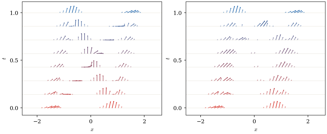
One-dimensional positive $\RR_+^2$-valued transport displayed by arrow glyphs at eight time levels. Each endpoint is a mixture of two localized Gaussian modes, and, inside each mode, both channel profiles have the same center. Each arrow is proportional to the local fiber value $(u_t^1(x),u_t^2(x))$, and time runs vertically from the red source to the blue target. Left: for $\kappa=0$, the diagonal mobility gives two independent scalar quantile geodesics. Right: a large-$\kappa$ common-mode interpolation bends the display toward $q=2^{-1/2}(1,1)$, illustrating the effect of a mobility that favors coherent channel motion while keeping the same componentwise continuity equation.

The interactive demo keeps the same glyph idea and lets the coupling strength bend the fibers toward a common channel direction.

Positive Matrix-Valued Measures¶

The next simplest fiber is the positive matrix cone. This is the simplest tensor-valued model beyond vectors: the diagonal entries behave like positive channels, while the eigenvectors encode local orientations.

If $\mathcal A$ has density $A(x)\succeq0$, then $\operatorname{tr}A(x)$ is the scalar amount of mass at $x$, while, wherever $\operatorname{tr}A(x)>0$, the normalized matrix $A(x)/\operatorname{tr}A(x)$ records an internal covariance or orientation. This is the matrix analogue of the positive vector case: diagonal matrices encode nonnegative vector components, and non-diagonal matrices add a local eigenbasis.

The conservative Benamou--Brenier model fixes a matrix density $A_t(x)\in\mathbb S_+^m$ and symmetric matrix fluxes $P_t(x)=(P_{t,1},\ldots,P_{t,d})\in(\mathbb S^m)^d$. With no flux through the boundary of $\X$, the full matrix mass $\int_\X A_t(x)\d x$ is conserved, so the endpoints must have the same total matrix. The model minimizes the matrix-perspective action

subject to $A_0\d x=\mathcal A_0$, $A_1\d x=\mathcal A_1$ and to the matrix-valued continuity equation

Here $A^\dagger$ denotes the Moore--Penrose inverse, with the usual perspective convention: the action is finite only when the columns of each $P_{t,\ell}$ belong to the range of $A_t$. The map $(A,P)\mapsto\operatorname{tr}(P^\top A^\dagger P)$ is the matrix fractional function and is jointly convex on $A\succeq0$. This gives the simplest non-trivial matrix-valued transport model: spatial motion is conservative, but the fiber carries orientation through the eigenvectors of $A_t(x)$.

The restriction to a fixed diagonal basis gives eigenvalue transport; it should be read as a commuting submodel, not as a claim that non-diagonal excursions can never change the unrestricted value. The genuinely matrix-valued case starts when the eigenspaces vary with $x$ or along the interpolation, so that the transported object carries both mass and orientation. Static matrix-valued Monge--Kantorovich problems and dual test-function metrics were developed in Ning & Georgiou, 2014Jiang et al., 2012Ning et al., 2015; dynamic versions and related non-commutative geometries appear in Chen et al., 2016Chen et al., 2020Carlen & Maas, 2014Peyré et al., 2019. The figure below shows the analogous independent/coupled contrast for positive $2\times2$ matrix fibers, using two localized matrix modes whose eigenvalue profiles share a common center at each mode.

show_book_figure("matrix-valued-measure-geodesic")

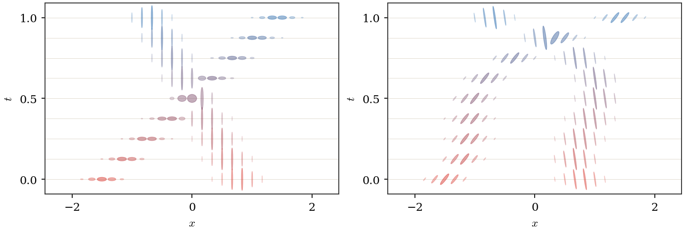
Positive $2\times2$ matrix-valued transport on a one-dimensional base. Each endpoint is a mixture of two localized matrix modes; within one mode, both eigenvalue profiles are Gaussian bumps with the same center. Each ellipse is the glyph of a positive semidefinite matrix $A_t(x)$, with axes given by eigenvectors and eigenvalues. Left: the matrices are diagonal in a fixed basis, giving the commuting tensor analogue of independent vector channels. Right: a coupled illustrative interpolation bends packet motion toward the trace-density transport and uses non-commuting eigendirections; the superposition remains positive semidefinite and produces spatially varying orientations.

Gromov--Wasserstein¶

Gromov--Wasserstein compares spaces through their internal distance structures rather than through a fixed ambient ground cost. This is the right extension for graphs, shapes and point clouds whose points are not pre-aligned.

Discrete Formulation¶

Optimal transport needs a ground cost $C$ to compare histograms $(a,b)$, and thus cannot be used directly if the histograms are not defined on the same underlying space, or if one cannot pre-register these spaces to define a ground cost. Instead, assume that two matrices $D\in\RR^{n\times n}$ and $D'\in\RR^{m\times m}$ represent relationships between points. A typical scenario is when these matrices are powers of distance matrices. The discrete Gromov--Wasserstein problem reads

where $p\geq1$ and $\Delta$ is usually $\Delta(u,v)=|u-v|$. This is a non-convex quadratic problem over the transport polytope. In the uniform case with $m=n$ and $P$ constrained to be a permutation matrix, it becomes a Quadratic Assignment Problem, already NP-hard in full generality Loiola et al., 2007. The relaxed coupling formulation can therefore be read as a soft graph-matching model Lyzinski et al., 2016.

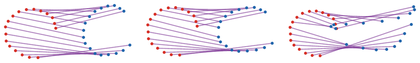
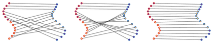
show_book_figure("gromov-isometry-matching")

Gromov--Wasserstein correspondences under increasing deformation. The red and blue point clouds are not compared through an ambient Euclidean cross-cost; instead, the GW coupling compares their internal pairwise distances. A perfectly isometric copy admits a clean structural match, while mild and deliberately stronger deformations progressively bend the correspondence.

The interactive demo uses a fixed structural correspondence and lets the deformation change the pairwise-distance residual. This isolates the quantity minimized by the GW objective.

When $D,D'$ are genuine distance matrices, the construction below defines a distance between metric spaces equipped with a probability distribution, up to measure-preserving isometries Mémoli, 2011Sturm, 2012Schmitzer & Schnörr, 2013. The same construction also explains why GW satisfies the triangle inequality after quotienting by isometries, and its relation to Hausdorff and Gromov--Hausdorff distances is discussed at the end of the section.

General Setting¶

The natural setting is that of Polish metric spaces; compactness is often assumed when one wants existence and a clean metric statement without adding tightness hypotheses.

For metric-measure spaces $\mathbb X=(\X,d_\X,\alpha)$ and $\mathbb Y=(\Y,d_\Y,\beta)$, define

The metric structure also gives geodesics. Sturm’s construction allows one to speak about interpolation, barycenters and gradient flows directly on the space of metric-measure spaces, even though the intermediate space lives on a product support and is therefore expensive numerically Sturm, 2012.

show_book_figure("gromov-nonisometric-distortion")

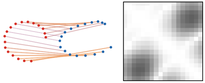
Local distortion in a mildly non-isometric GW match. The left panel colors transport segments by the average residual induced by the displayed hard correspondence. The right panel shows the pairwise-distance residual matrix $|d_\X(x_i,x_{i'})-d_\Y(y_{\sigma(i)},y_{\sigma(i')})|$, with darker entries marking larger local distortion. This matrix is the local contribution minimized by the discrete GW objective for the displayed correspondence.

This lower bound is useful computationally because the profile cost matrix $C_{ij}=\Wass_p(\alpha_{x_i},\beta_{y_j})^p$ is an ordinary OT cost between points. Solving this easier OT problem gives a geometry-aware initialization for the non-convex GW iterations; it is the same idea used above as a useful initialization principle for a non-convex solver.

Entropic Regularization and Fused GW¶

For the common squared distortion $\Delta(u,v)^2=(u-v)^2$, one often computes a stationary point of the entropic relaxation

Although the objective is non-convex, successive linearizations lead to a practical mirror-descent scheme Peyré et al., 2016. Up to an irrelevant global factor in the gradient, one alternates

with

Each update is an ordinary entropic OT problem and can therefore be solved with Sinkhorn iterations. This improves scalability and smooths the landscape, but it does not remove the non-convexity of the GW objective. This is the standard entropic GW solver used to compute soft maps between domains.

Fused Gromov--Wasserstein augments the structural term with a feature transport cost Vayer et al., 2019. In the discrete case, given a cross-feature cost $M\in\RR^{n\times m}$ and a parameter $\lambda\in[0,1]$, one minimizes

The endpoints $\lambda=0$ and $\lambda=1$ recover feature-only OT and pure GW respectively; intermediate values trade attribute matching against structural matching. The first term compares node attributes in the usual OT sense, and the second compares intrinsic geometry; this is useful when two spaces have both distances and features, and the two sources of information may disagree.

show_book_figure("fused-gromov-feature-geometry")

Feature information and intrinsic geometry in fused Gromov--Wasserstein. Small inner disks encode binary node features. Feature-only OT follows the attributes even when this crosses the shape structure, pure GW follows the intrinsic ordering, and fused GW balances the feature term with the pairwise-distance distortion.

Hausdorff and Gromov--Hausdorff Viewpoints¶

If $A,B$ are compact subsets of a common metric space $(\mathcal Z,d_\mathcal Z)$, their Hausdorff distance is

The Gromov--Hausdorff distance removes the common ambient space by minimizing this quantity over all isometric embeddings into a third space:

Equivalently, it is half the minimal distortion of a correspondence between $\X$ and $\Y$ Gromov, 2001Mémoli, 2007. This is a worst-case set distance: every point must be matched with small distortion. Gromov--Wasserstein replaces correspondences by probability couplings and worst-case distortion by averaged distortion. It is therefore better adapted to noisy sampled shapes and weighted graphs, but it can ignore small sets of mass that would dominate the Hausdorff distance.

Quantum Optimal Transport¶

Quantum optimal transport replaces probability vectors by density matrices and scalar couplings by positive operators on a tensor product space. This is the right language when the transported objects are matrix-valued signals, covariance-like descriptors or quantum states, and it exposes a precise bridge between OT, non-commutative entropy and operator scaling Ning & Georgiou, 2014Chen et al., 2016Chen et al., 2020Peyré et al., 2019Golse et al., 2019Chakrabarti et al., 2019.

Finite-Dimensional States and Couplings¶

A joint quantum state between $\mathbb C^n$ and $\mathbb C^m$ is a matrix $T\in\mathbb H_{nm}^+$ acting on $\mathbb C^n\otimes\mathbb C^m$. Its marginals are the partial traces, defined by duality through

for all $F\in\mathbb H_n$ and $G\in\mathbb H_m$. Thus $\operatorname{Tr}_B(T)\in\mathbb H_n^+$ and $\operatorname{Tr}_A(T)\in\mathbb H_m^+$ play exactly the role of the two marginals of a classical coupling.

The feasible set is never empty, since $A\otimes B$ has marginals $A$ and $B$.

The dual potentials have the usual scalar gauge freedom: replacing $(F,G)$ by $(F+tI_n,G-tI_m)$ leaves both the constraint and the value unchanged because $\operatorname{tr}(A)=\operatorname{tr}(B)=1$.

Entropic Regularization and Bregman Iterations¶

For $\epsilon>0$ define

This is the non-commutative analogue of entropic OT: the Shannon entropy of a coupling is replaced by the trace entropy of a density matrix Peyré et al., 2019Chakrabarti et al., 2019.

Writing $K=\exp(-C/\epsilon)$, the objective differs by a constant from $\epsilon$ times the quantum KL divergence

The exact quantum analogue of Sinkhorn is an implicit alternating Bregman projection scheme onto the affine marginal sets

In the diagonal case this proposition gives the usual multiplicative Sinkhorn updates. In the non-commutative case, however, the exact block equations

do not admit scalar division formulas, because the exponential of $F\otimes I_m+I_n\otimes G-C$ cannot be separated unless the local potential commutes with the cost.

Gurvits Scaling and Quantum Sinkhorn¶

The algorithm often called quantum Sinkhorn comes from the operator-scaling literature of Gurvits and subsequent developments Gurvits, 2003Gurvits, 2004Georgiou & Pavon, 2015Garg & Oliveira, 2018. It replaces the true Gibbs coupling (47) by the symmetric factorization

where $U=\exp(F/(2\epsilon))$, $V=\exp(G/(2\epsilon))$ and $K=\exp(-C/\epsilon)$. If $[Z,C]=0$, then $T_s(F,G)=T_e(F,G)$; otherwise this is a Strang-type symmetric surrogate.

Fix a Choi convention and let $\mathcal K:\mathbb H_m\to\mathbb H_n$ be the completely positive map represented by the positive Choi matrix $K$; let $\mathcal K^\star$ be its Hilbert--Schmidt adjoint. Up to the transpose dictated by the chosen Choi convention, the marginal equations for the symmetric coupling take the operator-scaling form

and can be enforced by the congruence normalizations

These inverse square roots are well-defined when $K\succ0$ and $U,V,A,B\succ0$. This is Gurvits/operator scaling with prescribed targets; when all matrices are diagonal it reduces to classical Sinkhorn scaling, and when the targets are proportional to identities it matches the usual bistochastic operator-scaling normalization, up to the conventional trace normalization.