The preceding gradient-flow calculus is variational. Modern machine-learning
models often use the same transportation language more broadly: one may
prescribe an interpolation and regress its velocity, fit a one-step generator
to a descent field, or view network depth as a continuous transport of token
measures. The examples below separate what is genuinely a Wasserstein gradient
flow from what is a transportation dynamics with a useful geometric
interpretation.
from pathlib import Path
import sys

from IPython.display import Image as DisplayImage
from IPython.display import display

here = Path.cwd()
myst_dir = None
for candidate in [here, here.parent, here / "myst", here.parent / "myst", here.parent.parent / "myst"]:
    if (candidate / "ot4ml_web.py").exists():
        myst_dir = candidate.resolve()
        sys.path.insert(0, str(myst_dir))
        break

if myst_dir is None:
    raise RuntimeError("Could not locate myst/ot4ml_web.py")

repo_root = myst_dir.parent
thumbnails = repo_root / "notebooks-figures" / "thumbnails"

def show_book_figure(name, width=760):
    display(DisplayImage(filename=str(thumbnails / f"{name}.png"), width=width))
Flow matching constructs a generative map by learning the velocity field of an interpolation. The key computational insight is that a constrained continuity-equation problem can be trained by an unconstrained regression.
Generative models aim to build a transportation map T between a reference distribution α (typically an isotropic Gaussian) and the target data distribution β. Since such reference measures are non-atomic, a measurable map with T♯α=β exists on standard Borel spaces, for instance by identifying both probability spaces with the unit interval and using a quantile-type rearrangement. This abstract existence statement is much weaker than having an explicit and numerically stable construction of T. Optimal transport is one approach to achieving this, but it is computationally expensive and raises questions about how to estimate it from samples. A different route is to prescribe an interpolation between noise and data, learn its velocity, and obtain T by integrating a time-dependent vector field vt. This point of view sits at the meeting point of two literatures, surveyed from a transport perspective in Peyré, 2025. The diffusion branch builds on score matching Hyvärinen, 2005, denoising score matching Vincent, 2011, nonequilibrium noising chains Sohl-Dickstein et al., 2015, denoising diffusion probabilistic models Ho et al., 2020, score-based generative modeling Song & Ermon, 2019, and the continuous-time score-SDE/probability-flow formulation Song et al., 2021. The deterministic regression branch was introduced, essentially in parallel, under three closely related names: flow matching Lipman et al., 2023, rectified flow Liu et al., 2023, and stochastic interpolants Albergo et al., 2025. In all three cases, the computational object is a velocity field whose regression loss avoids simulating the learned ODE during training. This vector field vt is obtained by constructing an interpolation αt and then finding vt using the least-squares formula of the dynamic chapter. As we will explain, for a specific class of interpolation (obtained by a parametric push-forward), this vt can be obtained by avoiding explicitly inverting a Laplacian and instead computing a simple conditional expectation. This conditional expectation can itself be estimated by solving another least-squares problem, but this time unconstrained, making the estimation feasible from finite samples of α and β.
A common case is d′=2d. We write (x,y)∈Rd′=Rd×Rd and assume P0(x,y)=x and P1(x,y)=y, so that π is a probabilistic coupling between α0 and α1, i.e. π has marginals (α0,α1). For instance, one can use π=α0⊗α1, the trivial coupling. An even more special case is the linear interpolation Pt(x,y)=(1−t)x+ty. With this linear path and an arbitrary coupling π, the regression below is the common core of flow matching and rectified flow: Lipman et al. emphasize conditional probability paths and simulation-free training of continuous normalizing flows, while rectified flow emphasizes straight couplings, reflow, and the possibility of reducing transport costs and discretization error Lipman et al., 2023Liu et al., 2023. More complex constructions are also possible, provided that sampling from π remains simple; stochastic interpolants allow additional latent variables and stochastic perturbations, thereby unifying deterministic flows, probability-flow ODEs and diffusion SDEs Albergo et al., 2025.
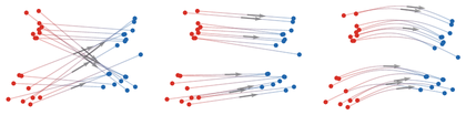
If π=α⊗β and α=n1∑iδxi, β=m1∑jδyj, then αt consists of n×m Dirac masses
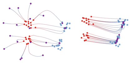
Flow matching interpolants between the same empirical source and target measures. A product-style random pairing produces crossing paths, an OT pairing gives direct displacement rays, and a curved bridge changes the path geometry while keeping the same endpoints. Gray arrows mark representative midpoint velocities ∂tPt.
Interactive panel. Use the interpolation and noise controls to compare flow-matching paths between source noise and target structure.
This interpolation is not directly useful for sampling from β, but it can be used to define a flow field vt so that the continuity equation, in Eulerian form, holds. This flow field is computed by solving an unconstrained least-squares problem, or equivalently, it is a conditional expectation.
Proof
We first recall the two equivalent ways of writing the interpolated measure. Formally, one may write
The minimizer in (3) is the orthogonal projection in L2(π;Rd) of the latent velocity ∂tPt(u) onto the closed subspace of functions that depend on u only through Pt(u). This projection is the conditional expectation (4). Formally, this can be read as
for every bounded continuous vector field ψ. Since αt(A)=0 implies π(Pt−1(A))=0, one has mt≪αt. The Radon--Nikodym decomposition of mt with respect to αt is therefore
In the language of Lebesgue decomposition, the flux measure mt has only an absolutely continuous part with respect to αt and no singular part; the conditional expectation is precisely this density. Equivalently, disintegrating π with respect to the map Pt gives π(du)=πt,z(du)αt(dz), where πt,z is supported on the fiber {u:Pt(u)=z}, and
Thus the solution of (3) is the conditional expectation of the velocities ∂tPt: intuitively, vt(z) is the average velocity of all trajectories passing through z. Numerically, (x,t)→vt(x) can be parameterized by a neural network (e.g., a U-Net for vision tasks) and estimated using stochastic gradient descent on the objective in (3). For the exact field vt, integrating the ODE x˙=vt(x) defines a transport map Tt. If vt is regular enough, or more generally if the continuity equation has a unique solution for this velocity, then (Tt)♯α0=αt. Thus the same interpolation as (1) is represented by a deterministic flow rather than by the original coupling. The sampling procedure consists in first drawing X0∼α, and then integrating the ODE X˙t=vt(Xt) starting with Xt=0=X0. In the ideal exact-field limit, the resulting Xt=1 is distributed according to α1=β.
In the special case where Pt(x,y)=(1−t)x+ty is a linear interpolation and π=α⊗β, the curve αt is a convolution of rescaled versions of α0 and α1. The flow-matching problem (3) becomes
When one endpoint is an isotropic Gaussian, this construction is closely related to the probability-flow formulation of diffusion models, up to the usual change of time parametrization Song et al., 2021. This is why flow matching can be viewed both as a deterministic alternative to diffusion training and as a common language for diffusion paths, OT-inspired paths, and rectified paths Lipman et al., 2023Liu et al., 2023Albergo et al., 2025. The next two propositions are written in the noising direction, from a data law α to a Gaussian; reversing time gives the corresponding sampling flow. They also give an explicit closed form for vt and show that it is a gradient field. In this setting, vt is also the solution of the constrained least-squares problem from the dynamic chapter. The regression (3) is computationally simpler because the continuity equation has already been enforced by the chosen interpolant. To prove this, we rely on Tweedie’s formula, which expresses the optimal Gaussian denoiser through the score, i.e. the gradient of the log-density.
Proof
Bayes’ rule gives the conditional density pW∣Z(w∣z)=βσ(z)β(w)φσ(z−w) with φσ the N(0,σ2Id) density. Hence
Fix t∈(0,1) and write W=(1−t)X, σ=t, so that Zt=W+σY matches the setting of Tweedie’s identity. Conditional expectations satisfy v⋆(z,t)=E[Y−X∣Zt=z]=t1E[Zt−W∣Zt=z]−1−t1E[W∣Zt=z]. Applying Tweedie’s identity to E[W∣Zt=z] and noting E[Y∣Zt=z]=−t∇logαt(z) gives the claimed formula.
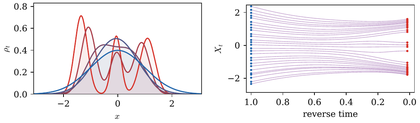
One-dimensional diffusion bridge for a Gaussian-mixture data law. The forward path Zt=(1−t)X+tY smooths the red data density toward a blue Gaussian endpoint. Reversing the probability-flow ODE transports a denser set of blue noise samples back toward the data modes, making the splitting of trajectories across mixture components visible.
Interactive panel. Use the noising time and schedule controls to see the one-dimensional forward and reverse diffusion bridge.
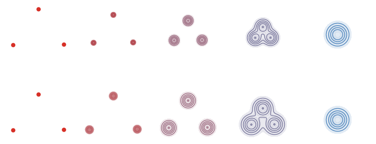
The same probability-flow intuition is visible in two dimensions. For a discrete data law, or more generally for a Gaussian mixture, the noising density is a Gaussian mixture whose score can be evaluated explicitly. This makes it possible to draw backward trajectories without training a neural network. In the plots below, the Gaussian endpoint has covariance σ2Id to keep the geometry visible at the scale of the three atoms. For a scalar noising schedule Zt=atX+btY, the intermediate law has component centers atcj and covariance (btσ)2Id. For the linear bridge, pt(z)=∑jwjN((1−t)cj,(tσ)2Id), with st=∇logpt, and the scaled Gaussian-endpoint field gives vt(z)=−(z+tσ2st(z))/(1−t).
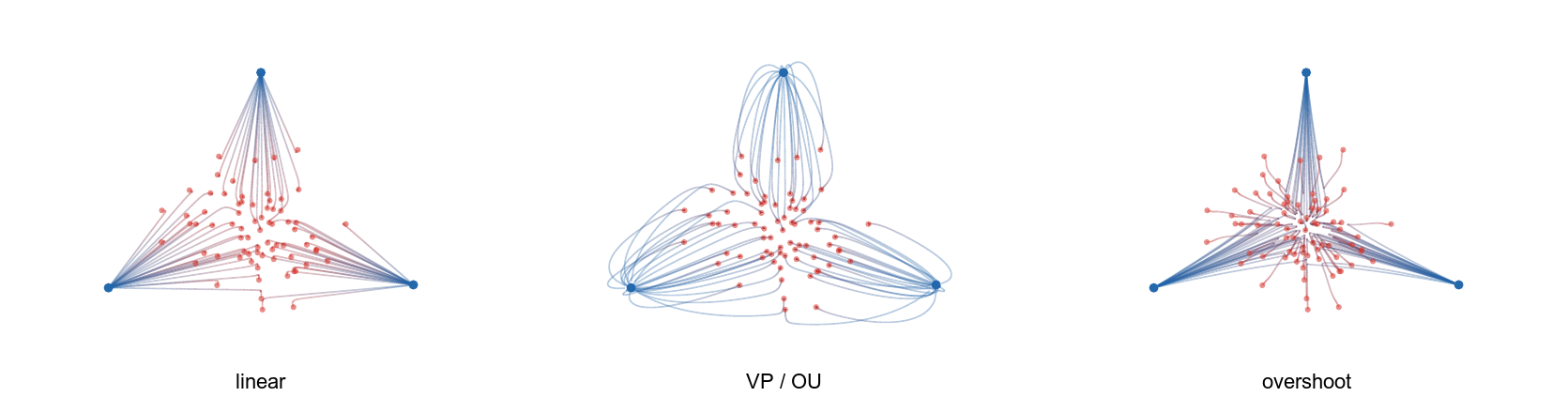
Two-dimensional noising paths from three Dirac masses to a single Gaussian. The linear interpolation Zt=(1−t)X+tY moves component centers linearly toward the origin and grows covariance like (tσ)2Id. The variance-preserving Ornstein--Uhlenbeck bridge has the same endpoints but a different speed of contraction and noising.
Interactive panel. Use the schedule and time controls to watch two-dimensional samples blur forward and concentrate backward.
Integrating the learned velocity gives a deterministic map from α0 to α1, but this map is not automatically the Brenier optimal map. It is optimal only in special cases where the accumulated flow remains the gradient of a convex potential. The Gaussian product-coupling case already shows the precise obstruction: the interpolated covariances are simple, the velocity is affine, but the terminal map can contain a hidden rotational part. This phenomenon, and its extensions to rectified flows and mixtures, is analyzed in depth in Hertrich et al., 2025.
which is exactly the equation T˙t=AtTt with T0=Id. Returning to the original coordinates gives (28), and t=1 gives (29).
Both T1FM and TOT push N(0,Σ0) to N(0,Σ1). The Brenier map between nondegenerate Gaussians is the unique symmetric positive definite linear map with this property. Hence T1FM=TOT if and only if T1FM is symmetric positive definite. The map T1FM is similar to C1/2, so if it is symmetric then it is automatically positive definite. It remains to characterize symmetry. Since C1/2 is symmetric positive definite,
Thus symmetry of T1FM is equivalent to Σ0C1/2=C1/2Σ0, hence to Σ0C=CΣ0 by functional calculus. Multiplying this identity on the left and right by Σ01/2 gives Σ0Σ1=Σ1Σ0. Conversely, if Σ0 and Σ1 commute, they are orthogonally co-diagonalizable, and both (29) and (30) reduce in that basis to the diagonal map with entries λ1,k/λ0,k. This proves the equivalence.
The Gaussian optimality proposition explains why the statement “flow matching gives an optimal map” is fragile. The same terminal map (29) is obtained for any scalar schedule Zt=atX0+btX1 with the same endpoints, because after whitening the covariance path remains at2Id+bt2C. Thus changing the speed of a scalar Gaussian bridge, for instance by using an OU schedule, cannot repair the non-optimality created by non-commuting covariances. Commuting covariances reduce the terminal map to independent one-dimensional scalings, whereas non-commuting covariances create a non-symmetric affine map, hence a transport with a rotational or shearing component. More generally, mixture-like paths can create the same obstruction even when every instantaneous velocity looks natural. This distinction is closely related to counterexamples showing that flow maps associated with Fokker--Planck or diffusion-type evolutions do not in general provide optimal transport maps Lavenant & Santambrogio, 2022. In particular, starting from an isotropic Gaussian does not by itself guarantee optimality once the target distribution is non-Gaussian; additional structural assumptions on the path or on the coupling are needed.
The geometry of the generated trajectories depends on the chosen interpolant, not only on the two endpoint laws. There is first a harmless ambiguity: a monotone reparametrization Zt=(1−λ(t))X+λ(t)Y of the linear bridge only changes the speed of the flow,
then both the mixture centers and the component variances are changed. Writing pt for the density of Zt and st=∇logpt, Tweedie’s formula gives, away from times where at=0,
For the linear bridge, at=1−t and bt=t, this recovers the formula above. For the variance-preserving Ornstein--Uhlenbeck noising used in diffusion models,
one obtains the forward probability-flow velocity vτ(z)=−z−σ2∇logpτ(z). Sampling follows the reverse field z+σ2∇logpτ(z) as τ decreases. This is the noising law used in the diffusion trajectory panel below; the trajectories are more curved than for the linear bridge because the centers and variances evolve according to the OU/Fokker--Planck scaling rather than by affine interpolation. Numerically, the integration is stopped at a small positive time before the Dirac endpoint, where the score becomes singular.
The finite-time coefficients at=cos(πt/2) and bt=sin(πt/2) are not a new spatial interpolant: they are exactly the OU coefficients after the time change τ=−logcos(πt/2). The schedule comparison below therefore places the OU bridge next to a genuinely different scalar bridge,
whose data coefficient changes sign before vanishing. This overshooting bridge is mainly a diagnostic example: it keeps the same endpoints, but its intermediate mixture reflects through the origin and produces visibly different reverse trajectories.
Diffusion-style sampling trajectories compared with OT rays in the three-Dirac setting. Red particles are sampled from the centered Gaussian endpoint and transported toward the three blue atoms. The diffusion panel integrates a reverse probability-flow field based on a Gaussian-mixture score, while the OT panel uses straight displacement rays selected by a quadratic matching.
Interactive panel. Use the trajectory and schedule controls to compare curved diffusion sampling paths with straight optimal-transport rays.
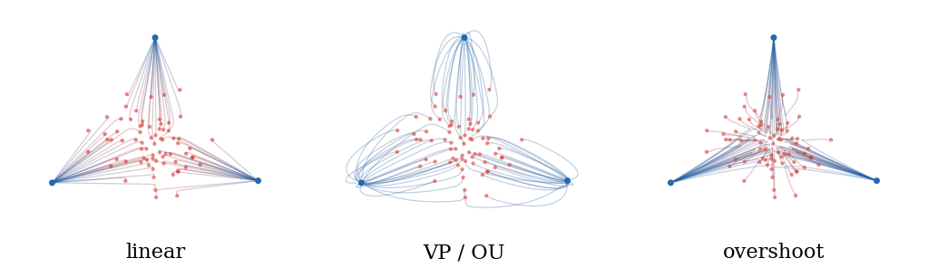
Effect of the interpolant on the exact reverse flow for the same three-Dirac target and the same Gaussian endpoint. The linear bridge at=1−t, bt=t produces almost radial curves. The variance-preserving OU bridge aτ=e−τ, bτ=1−e−2τ changes the relative speed of contraction and noising. The overshooting bridge at=(1−t)(1−2t), bt=t is not a time reparameterization of either one and produces a more pronounced bending of the reverse trajectories.
Interactive panel. Use the schedule controls to compare how different noising laws allocate motion over time.
One-step generative models try to keep the geometric training principle of flows while removing the expensive multi-step integration at sampling time. The idea is to evolve the model distribution during training, but to store the final evolution in a single generator evaluation.
Let ζ be a simple latent distribution and let αθ=(Gθ)♯ζ be the model distribution. Assume that the target data distribution is β. A Wasserstein-flow construction chooses a discrepancy
for instance a smoothed KL(α∣β), an MMD/IPM loss, or the debiased Sinkhorn divergence Lˉcϵ(α,β) introduced in the Sinkhorn divergence section. The associated formal descent is
After many training updates, the accumulated generator is evaluated once at test time. This is the organizing principle behind recent one-step methods based on Wasserstein gradient flows: W-Flow uses such a construction with the Sinkhorn divergence as a tractable global discrepancy Han et al., 2026, while drifting methods evolve the generated distribution during training through a fitted vector field and also admit one-step inference Deng et al., 2026. The gradient-flow interpretation of drifting models, and its relation to KL, MMD, sliced-Wasserstein and Sinkhorn-type discrepancies, is analyzed in Gretton et al., 2026He et al., 2026. These ideas are also connected to the Sinkhorn-type normalization dynamics used to model attention in Sinkformers Sander et al., 2022.
Drifting methods need not start from an exact Wasserstein gradient. They often prescribe an attraction-minus-repulsion field and then regress this field in L2(μt). A simple continuous version uses a positive kernel Kϵ(x,y) and defines, for any measure ν,
The first term pulls samples toward data, while the second term corrects self-attraction and prevents all particles from collapsing onto the same high-density region. Sinkhorn drifting replaces these one-sided kernel normalizations by two-sided entropic OT couplings, so that the cross and self terms are normalized by Sinkhorn scaling rather than by a single denominator He et al., 2026.
Drifting trajectories for a small particle generator. The raw kernel drift has weak long-range attraction and can leave particles away from the data modes. The self-corrected field uses the difference Bϵ[β]−Bϵ[μt], so a longer integration brings particles to the blue modes while repelling them from their own current concentration.
Interactive panel. Use the drift and time controls to inspect a learned-looking velocity field and its induced particle trajectories.
Proof
Since μt and ϕt are fixed in the variation with respect to α, the first variation is
The Wasserstein gradient-descent velocity is the negative of this gradient, namely ut. Substituting this velocity in the continuity equation gives the claimed flow.
Deep residual architectures can be read as time discretizations of ODEs or PDEs. For transformers, the transported objects are token measures and the velocity is induced by attention.
Transformers were introduced as sequence-to-sequence architectures driven by self-attention Vaswani et al., 2017 and have since become a central architecture for language and vision models Brown et al., 2020Dosovitskiy et al., 2021. Their distinctive feature is that each token is updated by a data-dependent average of all other tokens. This makes an attention layer permutation-equivariant before positional encoding, context dependent after conditioning on the input sequence, and naturally compatible with a measure viewpoint in which a prompt is regarded as an empirical distribution of tokens.
The mathematical limit used below concerns depth rather than model scale: one lets the number of residual attention layers grow while each layer makes a small update, as in continuous-depth neural networks Chen et al., 2018. For attention, the resulting velocity is nonlinear in the current token law because it is normalized by the whole context. This measure-theoretic view appears in the analysis of attention as a Lipschitz or interacting-particle operator Vuckovic et al., 2020Geshkovski et al., 2023, in the Sinkhorn-normalized dynamics of Sinkformers Sander et al., 2022, and in recent well-posedness and mean-field-limit results for several attention mechanisms Castin et al., 2025. It also separates the infinite-depth limit studied here from the token-limit question, where one controls how a finite empirical context approximates its limiting attention operator Bohbot et al., 2025.
We now consider very deep transformers, focusing on a single-head attention mechanism for simplicity while ignoring MLP layers, layer normalization, causality, and masking. This stripped-down framework is best suited to modeling encoders and vision transformers; the references above indicate which parts of this simplified picture extend to richer attention mechanisms.
After tokenization, embedding, and positional encoding, each input (from a set of tokens) is represented as a point cloud (xi)i=1n of n points in the space of vectorized tokens. An attention layer with skip connection and rescaling by 1/T (where T is the depth) defines a transformation of the tokens:
At the level of the token distribution, the layer pushes α forward by the “in-context” mapping Γθt[α], which depends on the context α, the tokens, and the depth-dependent parameters θt. Denoting t∈[0,1] as the depth and τ=1/T as the step size, this gives:
When the token space has dimension d and the query/key space has dimension r, take Q,K∈Rr×d and V∈Rd×d. If V=Q⊤K, the field Γθ[α] is a gradient vector field in the token variable. Indeed, define the log-partition potential
This is an instantaneous gradient in x. It is not, however, the gradient of the first variation of a fixed functional of α, because the potential Uα itself depends on the current measure through the same attention normalization. Thus the PDE is generally a transportation dynamics, not a Wasserstein gradient flow. Special variants recover additional structure: Sinkhorn attention can be interpreted through doubly stochastic normalization and Wasserstein-type gradient flows Sander et al., 2022Castin et al., 2025, while layer normalization leads naturally to dynamics on the sphere and to modified metrics. The key open difficulty for the present viewpoint is training: after the architecture has been rewritten as a controlled transport equation, learning corresponds to optimizing the time-dependent parameters (θt)t rather than merely analyzing the forward PDE for fixed parameters.
Gaussian measures provide a useful testing ground for the preceding dynamics. They are not invariant under a general Wasserstein gradient flow: a nonlinear velocity usually creates non-Gaussian densities immediately. The useful substitute is to either identify affine velocities, which exactly preserve Gaussianity, or to project the dynamics onto the Gaussian manifold. In both cases the measure PDE reduces to matrix ODEs for the mean and covariance. This viewpoint is emphasized in the survey Peyré, 2025 and is useful for comparing diffusion paths, Wasserstein gradient flows, drifting fields and transformer-type dynamics.
For constrained gradient flows on this family, the covariance equation is the finite-dimensional Bures--Wasserstein gradient flow on positive definite matrices. Thus Gaussian closure is not just a computational shortcut: it is the restriction of Wasserstein geometry to the Gaussian submanifold, where affine gradient fields encode tangent vectors.
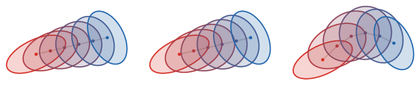
Gaussian closures of transport dynamics between two overlapping anisotropic Gaussians. The left panel is the exact W2 Gaussian geodesic. The middle panel shows a regularized Sinkhorn-style closure with inflated intermediate covariances. The right panel shows a drifting-style closure with a curved mean path and moment-matched covariance ellipses.
Interactive panel. Use the anisotropy, angle, regularization, and drift controls to compare Gaussian closures of Wasserstein, Sinkhorn, and drifting dynamics.
The first question is invariance: one wants a simple criterion ensuring that the continuity equation does not leave the finite-dimensional Gaussian family.
Proof
Let Xt follow the characteristic ODE X˙t=bt+At(Xt−mt). This linear ODE maps Gaussian random variables to Gaussian random variables. Taking expectation gives m˙t=bt. Writing X~t=Xt−mt, one has X~˙t=AtX~t, hence
For the converse, set bt=m˙t and choose any matrix At satisfying the covariance equation. Since Σt is positive definite, the Lyapunov map A↦AΣt+ΣtA is invertible on symmetric matrices, which gives the unique symmetric choice when a gradient velocity is required. In that case vt is the gradient of the quadratic potential x↦⟨bt,x⟩+⟨At(x−mt),x−mt⟩/2.
be the Gaussian submanifold of P2(Rd). The Wasserstein gradient of a functional constrained to a smooth submanifold M⊂P2 is defined as the Riesz representative of the differential restricted to tangent velocities of M. Equivalently, it is the small-step limit of the constrained JKO scheme
For M=G, tangent velocities are affine gradient fields v(x)=b+A(x−m) with A=A⊤. The constrained gradient is therefore the L2(N(m,Σ)) projection of the ambient Wasserstein gradient onto this finite-dimensional affine space, whenever the ambient gradient exists.
Proof
Test the functional along a Gaussian tangent vector, represented by an affine gradient field
for all affine gradient fields v. This identifies the constrained Wasserstein gradient in the induced L2(α) metric, or equivalently the projection of the ambient gradient when it exists. Substituting the descent velocity −vF in the affine-velocity moment equations gives (72).
This proposition should be read as the organizing rule for Gaussian closures: once the scalar energy has been reduced to a function of (m,Σ), its constrained Wasserstein gradient is automatically affine and the covariance follows the Bures-type ODE (72). When the first variation of f is quadratic, this constrained gradient coincides with the full Wasserstein gradient.
The next examples show that many familiar energies already have affine Wasserstein gradients on Gaussian inputs, so their full flow remains inside the Gaussian family.
Proof
Each row is obtained by identifying the affine descent velocity v(x)=MCx generated by the corresponding Gaussian-constrained calculation and then applying the affine covariance equation, which gives C˙=MCC+CMC⊤. For KL(⋅∣γ), the Fokker--Planck velocity is (C−1−Id)x, hence C˙=2(Id−C). For the Fisher row, the restriction of 21I to centered Gaussians is
Using the Gaussian-constrained gradient formula gives the descent velocity (C−2−Id)x, hence C˙=2(C−1−C). This row should be read as a Gaussian projected closure of the fourth-order Fisher flow.
For W22(⋅,γ), the Brenier map from N(0,C) to γ is C−1/2x, so the descent velocity for the unhalved squared distance is 2(C−1/2−Id)x, giving 4(C1/2−C). For the polynomial MMD row, centered Gaussians satisfy MMDk2(μ,γ)=∥C−Id∥F2; the first variation is quadratic and its descent velocity is 4(Id−C)x, giving 8(C−C2).
Gaussian Sinkhorn dual potentials are quadratic, so the velocity is again linear; differentiating the closed Gaussian formula yields the displayed spectral expression. The square roots are spectral functions of C, hence commute with C, which is why the covariance ODE closes as a matrix function of C alone. For sliced Wasserstein, each one-dimensional projection is a Gaussian transport with velocity 2((θ⊤Cθ)−1/2−1)⟨θ,x⟩θ; averaging these velocities over Sd−1 gives v(x)=V(C)x and thus C˙=V(C)C+CV(C).
The last examples are not ordinary gradient flows of a fixed scalar energy on the full Wasserstein space. They preserve Gaussianity because the prescribed velocity field is affine when evaluated on Gaussian measures.
The preceding examples show when Gaussianity is preserved or imposed by projection. Gelbrich’s inequality Gelbrich, 1990 gives a useful variational explanation: replacing a measure by the Gaussian with the same first two moments cannot increase its Wasserstein distance to another similarly projected measure.
Proof
Take any coupling (X,Y) of μ and ν, center the variables, and write C=E[(X−mμ)(Y−mν)⊤]. In the positive definite case, positivity of the block covariance matrix implies the factorization C=Σμ1/2KΣν1/2 with ∥K∥op≤1, and therefore, by operator/nuclear norm duality,
Taking the infimum over couplings proves the inequality, while equality for Gaussian laws is exactly the Gaussian Bures formula.
The following preservation criterion is a direct consequence of Gelbrich’s theorem and was explained to us by Hugo Lavenant. It says that a functional which does not increase under moment-matched Gaussian projection admits Gaussian minimizing movements from Gaussian initial data.
Proof
For the JKO claim, Rγ=γ because γ is Gaussian. Hence, for any competitor η,
Peyré, G. (2025). Optimal and Diffusion Transports in Machine Learning. arXiv Preprint arXiv:2512.06797.
Hyvärinen, A. (2005). Estimation of Non-Normalized Statistical Models by Score Matching. Journal of Machine Learning Research, 6, 695–709.
Vincent, P. (2011). A Connection Between Score Matching and Denoising Autoencoders. Neural Computation, 23(7), 1661–1674.
Sohl-Dickstein, J., Weiss, E. A., Maheswaranathan, N., & Ganguli, S. (2015). Deep Unsupervised Learning Using Nonequilibrium Thermodynamics. Proceedings of the 32nd International Conference on Machine Learning, 37, 2256–2265.
Ho, J., Jain, A., & Abbeel, P. (2020). Denoising Diffusion Probabilistic Models. Advances in Neural Information Processing Systems, 33, 6840–6851.
Song, Y., & Ermon, S. (2019). Generative Modeling by Estimating Gradients of the Data Distribution. Advances in Neural Information Processing Systems, 32.
Song, Y., Sohl-Dickstein, J., Kingma, D. P., Kumar, A., Ermon, S., & Poole, B. (2021). Score-Based Generative Modeling through Stochastic Differential Equations. International Conference on Learning Representations.
Lipman, Y., Chen, R. T. Q., Ben-Hamu, H., Nickel, M., & Le, M. (2023). Flow Matching for Generative Modeling. International Conference on Learning Representations.
Liu, X., Gong, C., & Liu, Q. (2023). Flow Straight and Fast: Learning to Generate and Transfer Data with Rectified Flow. International Conference on Learning Representations.
Albergo, M. S., Boffi, N. M., & Vanden-Eijnden, E. (2025). Stochastic Interpolants: A Unifying Framework for Flows and Diffusions. Journal of Machine Learning Research, 26(209), 1–80.
Hertrich, J., Chambolle, A., & Delon, J. (2025). On the Relation between Rectified Flows and Optimal Transport. Advances in Neural Information Processing Systems.
Lavenant, H., & Santambrogio, F. (2022). The Flow Map of the Fokker–Planck Equation Does Not Provide Optimal Transport. Applied Mathematics Letters, 133, 108225.
Han, J., Li, P., Guo, Q., Xu, R., Ermon, S., & Candès, E. J. (2026). One-Step Generative Modeling via Wasserstein Gradient Flows. arXiv Preprint arXiv:2605.11755.
Deng, M., Li, H., Li, T., Du, Y., & He, K. (2026). Generative Modeling via Drifting. arXiv Preprint arXiv:2602.04770.
Gretton, A., Li, K. W., Galashov, A., Thornton, J., De Bortoli, V., & Doucet, A. (2026). On the Wasserstein Gradient Flow Interpretation of Drifting Models. arXiv Preprint arXiv:2605.05118.