Entropic regularization makes optimal transport smooth, strictly convex and
scalable. This chapter first explains the discrete KL-regularized problem,
derives Sinkhorn’s alternating matrix scaling algorithm, and then rewrites the
same construction as a relative-entropy projection problem. It then records
the general continuous formulation, explains the path-space Schrodinger
problem behind the static coupling formulation, develops the dual
soft-transform picture, and presents the main convex regularization variants
and the debiased Sinkhorn divergence.
Entropy turns a possibly non-unique linear program into a unique smooth
problem. The price is bias, but the reward is differentiability and fast
scaling algorithms.
Using this entropy as a regularizing function gives the approximate transport
value
Equivalently, the regularizer is
ϵ∑i,jPi,jlogPi,j. It penalizes concentrated couplings
and makes the objective strictly convex on the relative interior of the
transport polytope.
Proof
The transport polytope is non-empty and compact, and the objective is
continuous with the convention 0log0=0, so a minimizer exists. On the
relative interior,
is positive definite on every non-zero feasible direction. Hence
−H is strictly convex on the polytope, which gives uniqueness.
If ai,bj>0 and a minimizer had Pi,j=0, then the perturbation
Pt=(1−t)P+ta⊗b remains feasible for small t>0. The derivative
of rlogr at zero along a positive direction is −∞, so the objective
decreases, contradicting optimality.
The entropy acts as a barrier for positivity and makes
LCϵ(a,b) smooth in a, b, and C as long as these
variables stay in the relative interior. As ϵ→+∞, the
minimizer converges to the independent coupling a⊗b; as
ϵ→0, it approaches the optimal face of the original transport
linear program.
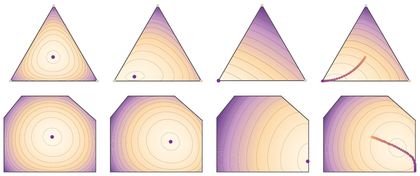
show_book_figure("sinkhorn-entropy-lp-geometry")
Entropic regularization and slack barriers. Large ϵ selects an
interior reference point, while small ϵ moves the minimizer toward a
low-cost face of the transport polytope. The second row gives the analogous
entropy-on-slacks picture for a generic linear program.
For a generic linear program minzℓ⊤z with constraints
Az≤b, one can introduce positive slacks s=b−Az and penalize them by an
entropy. This is a useful analogy, but it is not the standard self-concordant
interior-point barrier. The canonical barrier is the Burg, or reverse-KL,
barrier −∑ilogsi, which leads to Newton systems.
Optimal transport is special because entropy is placed on the entries of
P, while the constraints are only row and column marginals. This separable
structure turns Bregman projections into diagonal rescalings, giving the
Sinkhorn iterations.
Sinkhorn’s algorithm is alternating normalization of rows and columns. The
key point is that the optimizer of the entropic problem has a multiplicative
scaling form.
Proof
After removing zero-mass rows and columns, the minimizer is strictly positive,
so the positivity constraint can be ignored in the first-order conditions.
Introduce Lagrange multipliers f∈Rn and g∈Rm for the two
marginal constraints. The Lagrangian is
The division is entrywise. The scaling vectors are not unique: multiplying
u by λ>0 and v by 1/λ leaves P unchanged.
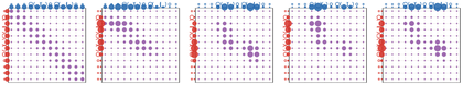
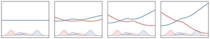
show_book_figure("sinkhorn-marginal-errors")
Marginal constraints during Sinkhorn scaling. Row normalizations align the
red source marginal and leave a blue defect; column normalizations align the
blue target marginal and leave a red defect.
The interactive demo exposes the alternating row/column normalization directly.
Change the half-step count to see the current coupling acquire one marginal,
lose the other, and then converge toward both.
Interactive panel. Use the iteration, regularization, and mass controls to watch Sinkhorn row and column scalings enforce the marginals.
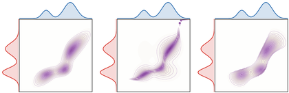
Dense Sinkhorn scaling for one-dimensional Gaussian-mixture marginals. The
violet side curves are the current row and column sums; the red and blue
curves are the prescribed marginals.
After convergence, the regularization strength controls how much of the Gibbs
kernel remains visible in the optimal plan. Small ϵ produces a
concentrated transport band, while larger ϵ spreads the same
marginals into a smoother coupling.
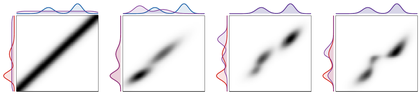
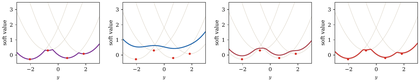
show_book_figure("sinkhorn-coupling-iterations")
Final Sinkhorn couplings for the same one-dimensional marginals and four
regularization strengths. Decreasing ϵ sharpens the plan toward an
optimal-transport graph; increasing ϵ keeps more of the product
structure.
KL-normalized dual potentials along the scaling iteration. The logarithmic
scaling potentials stabilize as the row/column normalizations converge.
The next interactive demo keeps the iteration count high and varies the temperature.
It is the quickest way to see the geometry-bias tradeoff: low temperature is
geometric and sharp, high temperature is smooth and closer to independence.
Interactive panel. Use the regularization slider to compare sparse exact-looking couplings with smoother entropic plans and potentials.
Complexity bounds for Sinkhorn and comparisons with accelerated first-order
methods are discussed in
Altschuler et al., 2017Dvurechensky et al., 2018Knight, 2008.
For a dense n×m problem, each iteration costs one multiplication by
K and one by K⊤, so the cost scales like Cnm for C iterations.
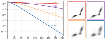
For fixed positive ϵ, the marginal error eventually has a linear
regime, but small ϵ makes the Gibbs kernel more peaked and scaling
harder.
show_book_figure("sinkhorn-linear-rate-epsilon")
Marginal violation along Sinkhorn half-steps for several values of
ϵ. Smaller ϵ gives sharper transport geometry but slower
scaling.
The KL formulation identifies Sinkhorn as a projection method. It also
prepares the continuous and unbalanced settings, where a reference measure is
essential.
For matrices with the same total mass, the affine terms cancel and
On fixed-mass couplings, taking Q=1n×m is equivalent to
subtracting the Shannon--Boltzmann entropy. Taking the tensor-product
reference gives the normalized formulation
The tensor-product reference is nevertheless useful when supports vary. It
makes explicit which entries may vanish and passes cleanly to the continuous
formulation.
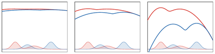
KL-normalized Sinkhorn dual potentials for one-dimensional Gaussian-mixture
histograms. Increasing ϵ turns the hard c-transform geometry into
smoother log-sum-exp potentials.
Proof Sketch
For ϵ→0, use compactness of the transport polytope and compare the
optimality inequalities for the entropic problem against an exact
Kantorovich optimizer. The cost gap is bounded by
ϵ times a KL difference, so every cluster point is cost-optimal; after
dividing by ϵ, the cluster point is the KL-minimizer on the optimal
face.
For ϵ→+∞, subtract a constant from C so that C≥0.
Testing the objective at a⊗b gives
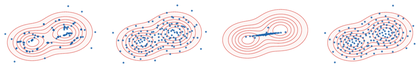
Entropically regularized couplings between the red disk and blue annulus
point clouds. The plans are strictly positive for every ϵ>0, but the
visible mass pattern evolves from nearly radial and sparse to diffuse as
ϵ increases.
For fixed balanced marginals, the specific product reference only matters up
to additive constants, provided the reference marginals are mutually
absolutely continuous with α and β. Its support still matters: it
determines which couplings have finite entropy.
Schrodinger’s reciprocal problem is naturally posed on paths rather than on
endpoint pairs. The Sinkhorn problem appears after the path law is reduced to
its two endpoint marginals.
Let Rϵ∈P(Ω) be a reference path law, for instance a
Brownian or Langevin dynamics at noise level ϵ. The dynamic
Schrodinger bridge problem is the entropy projection
It asks for the most likely path law, relative to the prior dynamics, among
all path laws matching the observed endpoints
Schrödinger, 1931Léonard, 2012Léonard, 2014Chen et al., 2016.
The dynamic problem also has viscous Benamou--Brenier formulations. In one
common convention,
After rewriting this prior with respect to α⊗β, the endpoint
problem is exactly the continuous Sinkhorn problem up to an additive constant.
Sinkhorn computes which endpoints should be paired; the path-space
Schrodinger bridge then connects each pair by a Brownian bridge.
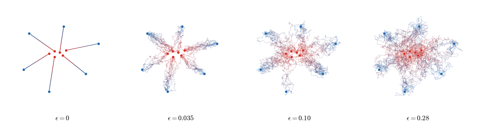
show_book_figure("sinkhorn-path-space-bridges")
Endpoint couplings lifted to Brownian bridges. Increasing ϵ both
softens the endpoint coupling and amplifies the Brownian fluctuations between
paired endpoints.
Large ϵ favors nearly independent endpoints, while small ϵ
suppresses endpoint randomness and recovers an optimal Monge--Kantorovich
coupling in the limit.
The dual point of view replaces couplings by potentials and soft
c-transforms. It is the right formulation for stabilized implementations
and differentiation.
Exponentiating the alternating soft-transform iterations recovers Sinkhorn’s
algorithm. For small ϵ, one must compute the log-sum-exp terms with
the usual stabilization trick: subtract the minimum before exponentiating and
add it back afterward.
This is the smooth counterpart of the hard feasibility constraint
f⊕g≤c from the Kantorovich dual.
Proof Sketch
Normalize potentials by imposing ∫fdα=0. Replacing a pair of
potentials by the corresponding soft transforms does not decrease the dual
objective. The transformed potentials have oscillations bounded by the
oscillation of c, and their modulus of continuity is controlled by the
modulus of continuity of c. Arzela--Ascoli gives existence.
Uniqueness up to constants follows from strict convexity of
H↦∫eH/ϵd(α⊗β) on the image of
(f,g)↦f⊕g−c, modulo constants.
KL regularization is the case that leads to multiplicative Sinkhorn scalings.
Replacing KL by another density-ratio penalty keeps the same transport
constraints but changes the scalar law linking the optimal density to the
dual potentials.
Density-ratio regularizers and coupling support. KL gives the usual diffuse
positive plan, the Burg barrier keeps positive but differently tailed support,
and the quadratic density penalty can set entries exactly to zero through its
positive-part law.
The interactive demo below separates the two effects. The left plot shows the
pointwise law r=h(s), while the right plot recomputes a coupling after
enforcing the marginals with that law. Changing ϵ controls how much
the cost score is softened; changing the regularizer changes whether mass is
spread everywhere, protected by a barrier, or clipped to a sparse support.
Interactive panel. Use the regularization-family and strength controls to compare entropic and quadratic penalties on the same transport problem.
The previous construction regularizes OT by a density-ratio divergence. This
differs from using a Bregman divergence generated by a convex functional on
the space of measures.
Main Idea of the Proof
Write the Bregman-regularized objective, up to constants independent of
π, as
Dualizing the marginal constraints and minimizing over π produces the
global conjugate Φ∗. Equality in Fenchel’s inequality gives the
Bregman optimality condition. The density-ratio dual follows instead from the
scalar Legendre formula for Dϕ(⋅∣α⊗β).
Thus the two generalizations lead to different duals and different
algorithms. Only for KL do density-ratio regularization and Bregman
projection geometry coincide and reduce to multiplicative Sinkhorn scalings.
Sinkhorn divergences remove the entropic self-bias while retaining
smoothness. They interpolate between OT-like geometry and kernel-like norms,
which explains their statistical behavior.
The raw Sinkhorn cost is biased: for ϵ>0, minimizing
Lcϵ(α,β) over β does not generally return
β=α. In the large-temperature limit, the raw value behaves like a
product interaction:
For c(x,y)=∥x−y∥2, minimizing this large-temperature limit over
β collapses toward a Dirac at the mean of α.
The standard debiasing subtracts the two self-interaction energies.
This cancellation removes the large-temperature attraction toward the
independent coupling; positivity is a separate property, proved below through
the positive-definite kernel associated with e−c/ϵ.
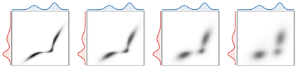
show_book_figure("sinkhorn-divergence-debiasing")
Debiasing by point optimization. For large ϵ, minimizing the raw
entropic cost collapses atoms toward the barycenter, whereas the self-cost
subtraction keeps a bimodal cloud.
The interactive demo below shows the same mechanism in a one-dimensional toy
setting. Move the model cloud relative to the target and compare the raw
entropic objective with its debiased version.
Interactive panel. Use the blur and separation controls to compare the raw entropic cost with the debiased Sinkhorn divergence.
for α-almost every x. Therefore the exponential penalty term in the
dual integrates to zero, and the dual value reduces to the two linear
potential terms.
Proof Sketch
Use the optimal self-potentials for (α,α) and (β,β) as
a suboptimal pair in the dual problem between α and β. After
rewriting with
α~=efα,α/ϵα and
β~=efβ,β/ϵβ, one obtains
Sinkhorn, R. (1964). A relationship between arbitrary positive matrices and doubly stochastic matrices. The Annals of Mathematical Statistics, 35(2), 876–879. 10.1214/aoms/1177703591
Sinkhorn, R., & Knopp, P. (1967). Concerning nonnegative matrices and doubly stochastic matrices. Pacific Journal of Mathematics, 21(2), 343–348. 10.2140/pjm.1967.21.343
Sinkhorn, R. (1967). Diagonal equivalence to matrices with prescribed row and column sums. American Mathematical Monthly, 74, 402–405.
Cuturi, M. (2013). Sinkhorn distances: lightspeed computation of optimal transport. Advances in Neural Information Processing Systems 26, 2292–2300.
Peyré, G., & Cuturi, M. (2019). Computational Optimal Transport with Applications to Data Sciences. Foundations and Trends in Machine Learning, 11(5–6), 355–607. 10.1561/2200000073
Altschuler, J., Weed, J., & Rigollet, P. (2017). Near-linear time approximation algorithms for optimal transport via Sinkhorn iteration. Advances in Neural Information Processing Systems, 30, 1964–1974.
Dvurechensky, P., Gasnikov, A., & Kroshnin, A. (2018). Computational Optimal Transport: Complexity by Accelerated Gradient Descent Is Better Than by Sinkhorn’s Algorithm. In J. Dy & A. Krause (Eds.), Proceedings of the 35th International Conference on Machine Learning (Vol. 80, pp. 1367–1376). PMLR.
Knight, P. A. (2008). The Sinkhorn–Knopp algorithm: convergence and applications. SIAM Journal on Matrix Analysis and Applications, 30(1), 261–275.
Schrödinger, E. (1931). Über die Umkehrung der Naturgesetze. Sitzungsberichte Preuss. Akad. Wiss. Berlin. Phys. Math., 144, 144–153.
Léonard, C. (2012). From the Schrödinger problem to the Monge–Kantorovich problem. Journal of Functional Analysis, 262(4), 1879–1920.
Léonard, C. (2014). A survey of the Schrödinger problem and some of its connections with optimal transport. Discrete Continuous Dynamical Systems Series A, 34(4), 1533–1574.
Chen, Y., Georgiou, T. T., & Pavon, M. (2016). On the relation between optimal transport and Schrödinger bridges: A stochastic control viewpoint. Journal of Optimization Theory and Applications, 169(2), 671–691.