Kantorovich Relaxation

Kantorovich’s relaxation is the decisive move that turns transport into convex optimization. Deterministic maps are replaced by couplings, infeasibility and asymmetry disappear, and the Wasserstein distances emerge. Historically, this linear-programming viewpoint grew from Kantorovich’s economic planning work Kantorovich, 1942 and is now the standard foundation of optimal transport Villani, 2003Villani, 2009Rachev & Rüschendorf, 1998.

from pathlib import Path
import sys

from IPython.display import Image as DisplayImage
from IPython.display import display

here = Path.cwd()
myst_dir = None
for candidate in [here, here.parent, here / "myst", here.parent / "myst", here.parent.parent / "myst"]:
    if (candidate / "ot4ml_web.py").exists():
        myst_dir = candidate.resolve()
        sys.path.insert(0, str(myst_dir))
        break

if myst_dir is None:
    raise RuntimeError("Could not locate myst/ot4ml_web.py")

repo_root = myst_dir.parent
thumbnails = repo_root / "notebooks-figures" / "thumbnails"

def show_book_figure(name, width=760):
    display(DisplayImage(filename=str(thumbnails / f"{name}.png"), width=width))

Discrete Relaxation¶

The discrete relaxation is the cleanest place to see mass splitting. It replaces permutations by a transportation polytope and reveals the linear-programming structure that algorithms exploit.

Monge’s discrete matching problem cannot be applied when the two clouds have different cardinalities or unequal weights. The continuous Monge problem has the same obstruction: there may be no map $T$ such that $T_\sharp\al=\be$ , for instance when one Dirac mass must be sent to several Dirac masses. It is also asymmetric: two Dirac masses can be mapped to one, but one Dirac mass cannot be split into two by a deterministic map.

Kantorovich’s idea is to relax deterministic transportation. Instead of sending each source point $x_i$ to exactly one target, the mass at $x_i$ may be dispatched across several targets. The relaxation is encoded by a coupling matrix $P\in\RR_+^{n\times m}$ for two discrete measures

\al=\sum_i a_i\delta_{x_i}, \qquad \be=\sum_j b_j\delta_{y_j}.

(1)

The first consequence is feasibility. There is always at least one admissible plan.

The feasible set is a bounded intersection of an affine space with the nonnegative orthant, hence a convex polytope. In one dimension, the coupling can be read as a matrix: rows index source bins, columns index target bins, and the marginal constraints appear as prescribed row and column sums.

Thus the product plan is mainly a feasibility witness. Except when the linear cost is constant on the whole transportation polytope, it is not expected to solve optimal transport.

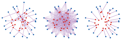
Discrete couplings represented as straight transport segments. The deterministic graph is a feasible Monge-type plan, the product plan spreads every source mass over all targets, and the optimal Kantorovich plan minimizes the quadratic transport cost. Line width and opacity encode transported mass.

The interactive demo below separates the main feasible-plan archetypes: deterministic graphs, independent product couplings, sparse splitting plans, and entropic approximations.

Interactive panel. Use the point and mass sliders to see how a Kantorovich plan can split mass into several weighted links rather than choosing one destination per source.

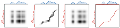
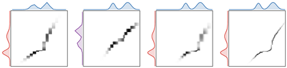
Coupling matrices with their prescribed marginals. The central grayscale image displays $P_{ij}$ ; the red curve on the left is the source marginal $a$ , and the blue curve on top is the target marginal $b$ . The independent product plan is diffuse, whereas the one-dimensional optimal plan concentrates near the monotone quantile correspondence.

The companion control varies the bin count and the endpoint laws, making the transition from diffuse independence to monotone transport visually explicit.

Interactive panel. Use the problem-size and mass-shape controls to compare the coupling matrix with its red and blue marginal sums.

The Kantorovich feasible set is symmetric: $P\in\CouplingsD(a,b)$ if and only if $P^\top\in\CouplingsD(b,a)$ . With a unit transport cost matrix $C_{ij}$ , the discrete Kantorovich problem reads

\mathcal{L}_C(a,b) \eqdef \min_{P\in\CouplingsD(a,b)} \langle C,P\rangle = \min_{P\in\CouplingsD(a,b)} \sum_{i,j} C_{ij}P_{ij}.

(7)

This is a linear program, and its solutions need not be unique.

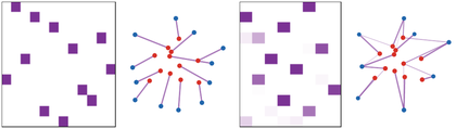
From permutation matrices to splitting couplings. When the two empirical measures have the same number of atoms and uniform weights, an optimal plan can be a permutation matrix. Once target masses are nonuniform, one source can send mass to several targets and several sources can merge into the same target.

The interactive demo keeps the same source and target sites while changing the target mass imbalance, so the moment where permutation structure breaks becomes visible.

Interactive panel. Use the split-mass and geometry controls to contrast deterministic permutation-like transport with plans that divide source mass across targets.

The north-west corner rule, summarized in Algorithm Algorithm: North-west corner coupling, does not use the cost matrix and is therefore not meant to solve the discrete Kantorovich problem. Its role is algorithmic: an acyclic support corresponds to linearly independent marginal constraints. When the support has fewer than $n+m-1$ positive entries, transportation simplex implementations complete it with zero-mass basic variables to obtain a degenerate basic feasible solution. This gives a cheap initialization for the pivoting methods discussed in Section Linear-Programming Algorithms.

One-Dimensional Cases¶

In one dimension, the transportation polytope has a canonical monotone optimizer. This is the weighted version of the sorting rule from the matching chapter.

Permutation Matrices As Couplings¶

Now assume $n=m$ and uniform weights $a=b=\mathbf{1}_n/n$ . In this case, a matching can be encoded as a matrix with exactly one active entry per row and per column.

The corresponding probability coupling is $P_\sigma/n$ . If the matching cost matrix is $C$ , then

\langle C,P_\sigma/n\rangle = \frac1n\sum_{i=1}^n C_{i,\sigma(i)}.

(12)

Thus the assignment problem is the minimization of a linear function over the discrete, non-convex set of permutation matrices. The convex relaxation replaces this finite set by all bistochastic matrices.

We first prove that permutation matrices are extreme. Let $P_\sigma\in\mathcal P_n^{\mathrm{perm}}$ and assume that

P_\sigma=\frac{Q+R}{2} \qquad\text{with}\qquad Q,R\in\mathcal B_n .

(16)

Every bistochastic matrix has entries in $[0,1]$ . Since the only extreme points of $[0,1]$ are 0 and 1, each entry of $P_\sigma$ fixes the corresponding entries of $Q$ and $R$ : if $(P_\sigma)_{ij}=0$ , then $Q_{ij}=R_{ij}=0$ , while if $(P_\sigma)_{ij}=1$ , then $Q_{ij}=R_{ij}=1$ . Hence $Q=R=P_\sigma$ , so $P_\sigma$ is extreme.

We now prove the converse by contrapositive. Pick $P\in\mathcal B_n\setminus\mathcal P_n^{\mathrm{perm}}$ . Since an integral bistochastic matrix is necessarily a permutation matrix, $P$ has at least one fractional entry. We shall split $P=(Q+R)/2$ with $Q,R\in\mathcal B_n$ and $Q\neq R$ , proving that $P$ is not extreme.

Associate with $P$ the bipartite graph whose left vertices are the rows, whose right vertices are the columns, and whose edges are the fractional entries $0<P_{ij}<1$ . An entry equal to 1 uses the whole mass of its row and column, so it is isolated in the positive support and does not appear in this fractional graph. If a left vertex is incident to one fractional edge, then it must be incident to at least one other fractional edge: after the first fractional contribution, the row still has positive remaining mass, and that remainder cannot be carried by an entry equal to 1. The same argument applies to columns. Thus every non-isolated vertex of the fractional graph has degree at least two.

Starting from any fractional edge, one may therefore walk through adjacent fractional edges without immediately backtracking and without getting stuck. Since the graph is finite, some vertex is eventually visited twice; the portion of the walk between the two visits contains a cycle. Choose a shortest such cycle and write it in alternating form

(i_1,j_1,i_2,j_2,\ldots,i_p,j_p), \qquad i_{p+1}=i_1,

(17)

where both $(i_s,j_s)$ and $(i_{s+1},j_s)$ are fractional for every $s$ . Define

\epsilon \eqdef \min_{1\leq s\leq p} \{ P_{i_s,j_s}, P_{i_{s+1},j_s}, 1-P_{i_s,j_s}, 1-P_{i_{s+1},j_s} \}>0,

(18)

and split the cycle edges into the alternating families

A=\{(i_s,j_s)\}_{s=1}^p, \qquad B=\{(i_{s+1},j_s)\}_{s=1}^p .

(19)

Set $Q=P$ and $R=P$ outside $A\cup B$ ; on $A$ , set $Q_{ij}=P_{ij}+\epsilon/2$ and $R_{ij}=P_{ij}-\epsilon/2$ ; on $B$ , set $Q_{ij}=P_{ij}-\epsilon/2$ and $R_{ij}=P_{ij}+\epsilon/2$ . By the definition of $\epsilon$ , all modified entries stay in $[0,1]$ . Each row and column of the cycle sees one $+\epsilon/2$ and one $-\epsilon/2$ , so the row and column sums remain one. Thus $Q,R\in\mathcal B_n$ , $Q\neq R$ , and $P=(Q+R)/2$ . Hence $P$ is not extreme. Consequently every extreme point of $\mathcal B_n$ is integral, and every integral bistochastic matrix is a permutation matrix.

The same combinatorial idea gives the constructive decomposition used to express a bistochastic matrix as a convex combination of permutations.

Algorithm: Birkhoff--von Neumann decomposition

Input: Bistochastic matrix $P\in\mathcal B_n$ .

Output: Decomposition $P=\sum_r\lambda_rP_{\sigma_r}$ .

Initialize: Set $R=P$ and $\mathcal L=\emptyset$ .

While $R\neq0$ do:

Build bipartite graph $G_R=\{(i,j):R_{ij}>0\}$ .
Set $\sigma$ to the lexicographically first perfect matching of $G_R$ .
Set $\lambda=\min_i R_{i,\sigma(i)}.$
Append $(\lambda,\sigma)$ to $\mathcal L$ .
Update $R\leftarrow R-\lambda P_\sigma .$

Return $P=\sum_{(\lambda_r,\sigma_r)\in\mathcal L}\lambda_rP_{\sigma_r}, \qquad \sum_r\lambda_r=1.$

Equivalently, for uniform empirical measures, one can always choose a permutation matrix among the minimizers of the relaxed Kantorovich problem: the relaxation is tight for assignment problems.

Linear-Programming Algorithms¶

The discrete Kantorovich problem is a linear program with much more structure than a generic dense LP. Its variables are arcs of a complete bipartite network, its equality constraints are flow-conservation constraints, and its extreme points are sparse tree-like couplings.

Transportation Simplex And Network Simplex¶

The transportation simplex goes back to Dantzig’s formulation of the transportation problem Dantzig, 1951. It works on basic feasible couplings, whose support is completed into a spanning tree of the bipartite supply-demand graph. Reduced costs identify whether an unused arc can decrease the objective. Adding such an arc creates a unique cycle; one then pushes as much mass as possible around that cycle and removes the exhausted arc.

The network simplex is the corresponding pivoting method for general minimum-cost-flow problems Bertsekas & Eckstein, 1988. It keeps node potentials, reduced costs and a spanning-tree basis. Its worst-case number of pivots can be exponential, but the per-pivot operations exploit graph sparsity. Polynomial guarantees can be obtained from strongly polynomial minimum-cost-flow algorithms such as Orlin’s algorithm Orlin, 1997.

Interior-Point Methods¶

Generic interior-point methods approach the LP through a smooth central path. For the transport polytope, the logarithmic-barrier version is

P_\epsilon \eqdef \argmin_{\substack{P\mathbf{1}_m=a,\;P^\top\mathbf{1}_n=b\\P_{ij}>0}} \langle C,P\rangle - \epsilon\sum_{i,j}\log P_{ij}.

(20)

The barrier is singular at the boundary, so each iterate stays strictly inside the transportation polytope. As $\epsilon\downarrow0$ , the central path approaches the set of LP minimizers.

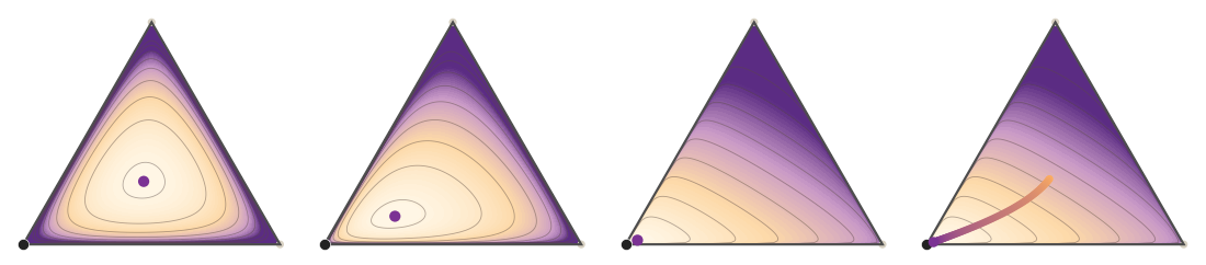
Logarithmic-barrier central path for a triangular slice of a linear program. Large $\epsilon$ selects a central interior point; decreasing $\epsilon$ moves the minimizer toward the optimal vertex while never touching the boundary. This differs from entropic OT, where the entropy temperature is part of the regularized objective itself.

The interactive view exposes the barrier parameter directly: lowering $\epsilon$ slides the minimizer from the center of the feasible triangle toward the LP vertex.

Interactive panel. Use the barrier and angle controls to move along the interior central path of the transport polytope.

Both interior-point methods and Sinkhorn keep iterates positive, but they use positivity differently. Interior-point algorithms solve the original LP by decreasing a barrier parameter. Sinkhorn fixes an entropic temperature and solves a different, KL-regularized OT problem by alternating diagonal scalings.

Relaxation For Arbitrary Measures¶

This section lifts the finite-dimensional coupling matrix to a joint probability measure. The payoff is that existence, duality and metric properties can be stated for arbitrary laws, including discrete, singular and continuous distributions.

Continuous Couplings¶

Remark: Probabilistic interpretation of couplings

If $X\sim\al$ and $Y\sim\be$ , then $\pi\in\Couplings(\al,\be)$ means that $\pi$ is the law of a pair $(X,Y)$ whose coordinates have laws $\al$ and $\be$ . The coupling encodes the dependence between $X$ and $Y$ . The tensor product $\al\otimes\be$ corresponds to independence, whereas a graph coupling $(\Id,T)_\sharp\al$ corresponds to the deterministic relation $Y=T(X)$ .

In the discrete case, when $\al=\sum_i \a_i\de_{x_i}$ and $\be=\sum_j \b_j\de_{y_j}$ , the constraint $\pi_1=\al$ and $\pi_2=\be$ forces every coupling to have the form $\pi=\sum_{i,j}\P_{ij}\de_{(x_i,y_j)}$ with $\P\in\CouplingsD(\a,\b)$ . The discrete formulation is therefore a special case of the continuous one, not merely an approximation.

Unlike the Monge constraint, the coupling constraint is never empty. The continuous feasibility witness is the tensor product coupling.

If there exists a map $T:\Xx\to\Yy$ with $T_\sharp\al=\be$ , then the Monge map induces the graph coupling $\pi=(\Id,T)_\sharp\al\in\Couplings(\al,\be)$ , characterized by

\int h(x,y)\d\pi(x,y) = \int h(x,T(x))\d\al(x).

(26)

Graph couplings are precisely the Kantorovich representation of deterministic Monge maps.

Continuous Kantorovich Problem¶

The discrete Kantorovich problem becomes, for arbitrary measures,

\mathcal{L}_c(\al,\be) \eqdef \inf_{\pi\in\Couplings(\al,\be)} \int_{\Xx\times\Yy} c(x,y)\d\pi(x,y).

(27)

This is an infinite-dimensional linear program over a space of measures.

On non-compact domains, one needs coercivity and moment conditions. For the Wasserstein cost $c(x,y)=d(x,y)^p$ on a Polish metric space, the natural domain is

\mathcal P_p(\Xx) \eqdef \left\{ \mu\in\Mm_+^1(\Xx): \int d(x,x_0)^p\d\mu(x)<+\infty \right\},

(29)

for one, and hence every, reference point $x_0$ .

Monge--Kantorovich Equivalence¶

The proof of Brenier’s theorem relies on Kantorovich relaxation and duality. Under Brenier’s hypotheses, the relaxation is tight: it has the same cost as the Monge problem and the optimal coupling is induced by a map.

If $\al$ does not have a density, non-smooth points of $\phi$ can be charged by $\al$ and mass splitting can occur. For instance, moving $\delta_0$ to $(\delta_{-1}+\delta_1)/2$ can be represented by a plan concentrated on the set-valued subdifferential of $\phi(x)=|x|$ , but not by a deterministic map.

Cyclical Monotonicity¶

Cyclical monotonicity is the local geometric fingerprint of optimality for a cost $c$ . It converts a global minimization problem into finite exchange inequalities and is the bridge from Kantorovich plans to convex potentials.

It is enough to check cyclic permutations:

\sum_{i=1}^k c(x_i,y_i) \leq \sum_{i=1}^k c(x_i,y_{i+1}), \qquad y_{k+1}=y_1.

(33)

If the optimal plan is induced by a map $T$ , cyclical monotonicity reads

\sum_{i=1}^k c(x_i,T(x_i)) \leq \sum_{i=1}^k c(x_i,T(x_{i+1})).

(34)

For $c(x,y)=\frac12\|x-y\|^2$ , the two-point case gives

\langle T(x)-T(y),x-y\rangle\geq0,

(35)

so $T$ is a monotone vector field. In one dimension, for $c(x,y)=|x-y|^p$ , this reduces to the classical monotone rearrangement.

Metric Properties: Wasserstein Distances¶

OT costs become genuine distances when the ground cost comes from a metric. The proof relies on a gluing lemma.

Discrete gluing lemma in matrix form. The first two panels are optimal one-dimensional couplings through an intermediate marginal. The third panel shows the induced marginal $R=P\diag(1/b)Q$ ; it is feasible and is the coupling used in the triangle-inequality proof.

The interactive version changes the resolution of the intermediate marginal, which controls how mediated the glued source-target plan becomes.

Interactive panel. Use the mediation slider to inspect how two couplings through an intermediate marginal glue into a source-target plan.

Interpolation Induced By A Plan¶

The quadratic Wasserstein distance does not only compare two endpoint measures. An optimal plan also says how to move mass between them: each active pair $(x,y)$ travels along the segment joining $x$ to $y$ . This turns an optimal coupling into a curve of measures.

In the discrete case, each mass $P_{ij}$ moves from $x_i$ to $y_j$ along its own segment. When the optimal plan is not induced by a map, one source atom can split into several moving atoms. If the optimal plan is not unique, different optimal plans may also induce different $\Wass_2$ geodesics.

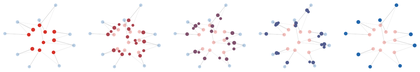
McCann interpolation induced by a non-deterministic optimal transport plan. In every panel, the red and blue endpoint measures are shown with low opacity, thin gray segments display the support $P_{ij}>\mathrm{tol}$ of the coupling, and the moving atoms are colored from red to blue along the interpolation.

The companion panel lets the same coupling be inspected along time $t$ , with an entropy slider to contrast sparse and diffuse plans.

Interactive panel. Use the interpolation time and plan controls to see how a fixed coupling induces a cloud of displacement paths between endpoint measures.

General Geodesic Spaces¶

For Dirac masses in Euclidean space, the $\Wass_2$ geodesic from $\delta_x$ to $\delta_y$ is $t\mapsto\delta_{(1-t)x+t y}$ . The same idea extends to any geodesic metric space $(\X,d)$ , meaning that each pair of points can be joined by a constant-speed metric geodesic. For each pair $(x,y)$ , one replaces the Euclidean segment by a curve $\gamma^{x,y}:[0,1]\to\X$ such that $\gamma^{x,y}_0=x$ , $\gamma^{x,y}_1=y$ , and

d(\gamma^{x,y}_s,\gamma^{x,y}_t)=|t-s|d(x,y).

(49)

If this geodesic is unique and depends measurably on $(x,y)$ , one defines $e_t(x,y)=\gamma^{x,y}_t$ and sets $\al_t=(e_t)_\sharp\pi^\star$ for an optimal coupling $\pi^\star$ . When geodesics are not unique, there is no canonical interpolation of a pair of Diracs unless a choice is made: one may select a particular geodesic between $x$ and $y$ , or randomize among several such geodesics. The intrinsic formulation is to choose a probability measure $\eta$ on the path space of constant-speed geodesics, called a dynamical optimal plan, such that $(e_0,e_1)_\sharp\eta$ is an optimal coupling, and to set $\al_t=(e_t)_\sharp\eta$ . Different measurable choices, or different conditional distributions over geodesics with the same endpoints, can give different $\Wass_2$ geodesics; the constant-speed identity remains the same. This path-space viewpoint is standard in the general theory of Wasserstein spaces Ambrosio et al., 2006Villani, 2009Santambrogio, 2015.

Comparison With Monge¶

The distance $\Wass_p$ defined through the Kantorovich problem (42) should be contrasted with the directed distance $\widetilde{\Wass}$ obtained using Monge’s problem. The Kantorovich feasible set is never empty, since it contains the product coupling, although the $p$ -cost may still be infinite without moment assumptions on non-compact spaces. By contrast, Monge’s constraint set $\{T:T_\sharp\al=\be\}$ can be empty. When an optimal Monge map exists, Kantorovich gives the same value by choosing the graph coupling $(\Id,T)_\sharp\alpha$ ; in this sense the Kantorovich problem is the convex relaxation of Monge’s problem, with much better stability properties.

Metric Properties: Topology And Applications¶

Wasserstein distances metrize weak convergence under moment control, sit between weak and strong topologies, and provide quantitative estimates in probability and robust optimization.

Remark: Weak convergence for discrete measures

In the special case of a single Dirac, $\de_{x^{(n)}} \rightharpoonup \de_x$ is equivalent to $\int f \d\de_{x^{(n)}} = f(x^{(n)}) \rightarrow \int f \d\de_{x} = f(x)$ for any continuous $f$ . This in turn is equivalent to $x^{(n)} \rightarrow x$ . For a fixed number of atoms, if $\al_n=\sum_{i=1}^N a_i^{(n)}\de_{x_i^{(n)}}$ and, after extracting a subsequence and relabeling, $a_i^{(n)}\to a_i$ and $x_i^{(n)}\to x_i$ , then $\al_n$ converges weakly to $\sum_i a_i\de_{x_i}$ , with atoms at identical limits merged. Without a uniform bound on the number of atoms, weak limits of discrete measures can be non-discrete; empirical measures are the standard example.

Remark: Modes of convergence for random variables

Convergence of laws should be distinguished from stronger notions of convergence for random variables. If $X_n$ and $X$ are defined on a common probability space, then $X_n\to X$ almost surely means pointwise convergence outside a null set, while convergence in probability means

\foralls \epsilon>0,\qquad \PP(\norm{X_n-X}>\epsilon)\to0.

(54)

Almost-sure convergence implies convergence in probability, and convergence in probability implies convergence in law. Convergence in law is exactly weak $^*$ convergence of the probability measures $(X_n)_\sharp\PP\rightharpoonup X_\sharp\PP$ , and does not require all variables to live on the same probability space. Strong convergence of measures, for instance convergence in total variation, is different and usually much stronger: it controls the mass assigned to all measurable sets, not only averages against continuous test functions. In particular, total variation convergence implies weak convergence, but the converse fails for empirical approximations of continuous laws.

For Dirac masses,

\|\delta_{x_n}-\delta_x\|_{\TV}=2, \qquad \Wass_p(\delta_{x_n},\delta_x)=d(x_n,x).

(57)

Thus the strong topology never sees Diracs converge unless they are eventually equal, while the Wasserstein topology captures their spatial convergence.

On non-compact spaces, one must also impose convergence of $p$ -th moments: $\Wass_p(\alpha_k,\alpha)\to0$ if and only if $\alpha_k\rightharpoonup\alpha$ and

\int d(x,x_0)^p\d\alpha_k(x) \to \int d(x,x_0)^p\d\alpha(x).

(58)

On a discrete space, weak and strong topologies coincide, and

\frac{d_{\min}}{2}\|\al-\be\|_{\TV} \leq \Wass_1(\al,\be) \leq \frac{d_{\max}}{2}\|\al-\be\|_{\TV}.

(59)

Wasserstein Over Wasserstein¶

The construction can be iterated. Once $(\X,d)$ is a metric space, the set of probability measures on $\X$ becomes a metric space through $\Wass_p$ . It can therefore serve as a new ground space. This is useful whenever the objects to compare are themselves random probability measures, or mixtures whose components are meaningful objects rather than only a collapsed density.

Elements of $\Pp_2(\Pp_2(\X))$ are probability laws over probability measures, or random probability measures. A parametric example is

\mathfrak A=(\zeta\mapsto\alpha_\zeta)_\sharp\gamma.

(60)

The Wasserstein distance on the Wasserstein space is

\mathbb W_2^2(\mathfrak A,\mathfrak B) \eqdef \inf_{\Pi\in\Couplings(\mathfrak A,\mathfrak B)} \int_{\Pp_2(\X)\times\Pp_2(\X)} \Wass_2^2(\alpha,\beta)\d\Pi(\alpha,\beta).

(62)

For Gaussian mixtures, this separates two geometries. A mixture can be viewed as a collapsed density on $\X$ , or as a component law over Gaussian atoms in the Bures--Wasserstein space. For two component laws

\mathfrak A=\sum_i a_i\delta_{\Gaussian(m_i,\Sigma_i)}, \qquad \mathfrak B=\sum_j b_j\delta_{\Gaussian(n_j,\Lambda_j)},

(63)

the component-level problem uses the cost

C_{ij}=\norm{m_i-n_j}^2+\Bb(\Sigma_i,\Lambda_j)^2.

(64)

If $\Pi^\star$ is an optimal coupling between the weights $a$ and $b$ , and if $A_{ij}$ is the Brenier linear part from $\Sigma_i$ to $\Lambda_j$ , each active pair follows the Gaussian geodesic

m_{ij,t}=(1-t)m_i+t n_j, \qquad \Sigma_{ij,t} = \big((1-t)\Id+tA_{ij}\big)\Sigma_i \big((1-t)\Id+tA_{ij}\big).

(65)

Collapsing these component geodesics gives

\bar\alpha_t= \sum_{i,j}\Pi^\star_{ij}\Gaussian(m_{ij,t},\Sigma_{ij,t}).

(66)

This component-level interpolation generally differs from the true $\Wass_2$ interpolation between the collapsed mixture densities.

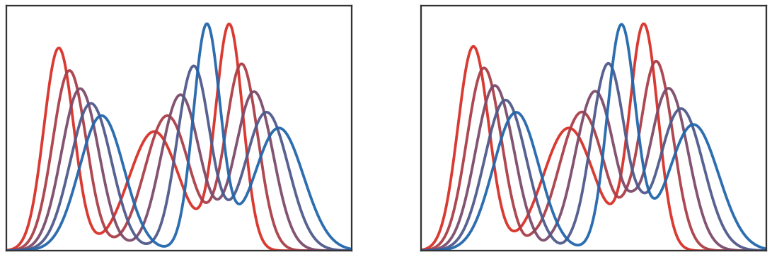
Two interpolations between the same three-component one-dimensional Gaussian mixtures. On the left, components are matched using the Bures--Wasserstein distance between Gaussians. On the right, the mixtures are collapsed into ordinary one-dimensional densities and interpolated by the true quantile formula for $\Wass_2$ .

The interactive comparison keeps both geometries side by side: component-level transport moves Gaussian atoms, while collapsed transport rearranges the full density.

Interactive panel. Use the mixture and blur controls to compare transport between ordinary measures with transport between distributions of measures.

This viewpoint also clarifies lower bounds for Gromov--Wasserstein distances: a metric-measure space can be mapped to a law of local distance profiles, and these laws can be compared by Wasserstein-over-Wasserstein.

Remark: Local profiles as Wasserstein-over-Wasserstein laws

Given a metric-measure space $\XX=(\X,\dist_\X,\mu_\X)$ , each point defines a local distance distribution

\alpha_x=(\dist_\X(x,\cdot))_\sharp\mu_\X\in\Pp(\RR_+), \qquad \mathfrak D_\X=(x\mapsto\alpha_x)_\sharp\mu_\X\in\Pp(\Pp(\RR_+)).

(68)

The Memoli profile lower bound in Proposition Proposition: Memoli Profile Lower Bound is precisely a Wasserstein-over-Wasserstein comparison of these laws of local profiles. It replaces the full pairwise distortion by an ordinary OT problem whose ground cost is itself a one-dimensional Wasserstein distance.

Note that there exist alternative distances which also metricize weak convergence. The simplest ones are Hilbertian kernel norms, which are detailed in Section Dual Norms and Integral Probability Metrics.

Distributional Robustness And Wasserstein Infinity¶

Wasserstein distances define ambiguity sets around empirical laws. Given samples $z_i$ and $\hat\alpha_n=\frac1n\sum_i\delta_{z_i}$ , a distributionally robust optimization problem replaces empirical risk by

\sup_{\beta:\Wass_p(\beta,\hat\alpha_n)\leq\rho} \int \ell_\theta(z)\d\beta(z).

(69)

Under standard upper-semicontinuity and growth assumptions on the loss, one has the dual reformulation

\sup_{\beta:\Wass_p(\beta,\hat\alpha_n)^p\leq\rho^p} \int \ell_\theta\d\beta = \inf_{\lambda\geq0} \lambda\rho^p + \frac1n\sum_{i=1}^n \sup_z\{\ell_\theta(z)-\lambda d(z,z_i)^p\}.

(70)

The robust risk is therefore an empirical risk in which each sample is replaced by its worst penalized perturbation. For $p=1$ and an $L_\theta$ -Lipschitz loss,

\sup_{\beta:\Wass_1(\beta,\hat\alpha_n)\leq\rho} \int \ell_\theta\d\beta \leq \frac1n\sum_i\ell_\theta(z_i)+\rho L_\theta.

(71)

The limiting distance

\Wass_\infty(\alpha,\beta) \eqdef \inf_{\pi\in\Couplings(\alpha,\beta)} \esssup_{(x,y)\sim\pi} d(x,y)

(73)

minimizes the worst displacement rather than an average displacement.

Theoretical Application: Quantitative Central Limit Theorems¶

Weak topology says whether laws converge; Wasserstein distances also quantify how fast. The central limit theorem becomes a rate estimate in $\Wass_1$ , which controls the error of all 1-Lipschitz observables of the normalized sum.

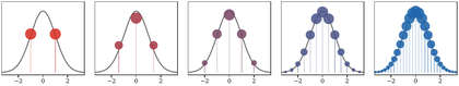
Central-limit theorem for normalized Bernoulli sums. Starting from $\alpha_0=\frac12(\delta_{-1}+\delta_1)$ , the law of $Z_n=n^{-1/2}\sum_i X_i$ remains discrete, but its rescaled atom heights approach the standard Gaussian density shown in gray.

The interactive demo varies the number of summands and the Bernoulli skew, making the Wasserstein view of weak convergence visible even while the law remains discrete.

Interactive panel. Use the dimension and sample-size controls to watch the Wasserstein CLT scaling predicted by Lipschitz test functions.

References¶

Kantorovich, L. (1942). On the transfer of masses (in Russian). Doklady Akademii Nauk, 37(2), 227–229.
Villani, C. (2003). Topics in Optimal Transportation (Vol. 58). American Mathematical Society.
Villani, C. (2009). Optimal Transport: Old and New (Vol. 338). Springer.
Rachev, S. T., & Rüschendorf, L. (1998). Mass Transportation Problems: Volume II: Applications. Springer.
Dantzig, G. B. (1951). Application of the simplex method to a transportation problem. Activity Analysis of Production and Allocation, 13, 359–373.
Bertsekas, D. P., & Eckstein, J. (1988). Dual coordinate step methods for linear network flow problems. Mathematical Programming, 42(1), 203–243.
Orlin, J. B. (1997). A polynomial time primal network simplex algorithm for minimum cost flows. Mathematical Programming, 78(2), 109–129.
Ambrosio, L., Gigli, N., & Savaré, G. (2006). Gradient Flows in Metric Spaces and in the Space of Probability Measures. Springer.
Santambrogio, F. (2015). Optimal Transport for Applied Mathematicians: Calculus of Variations, PDEs, and Modeling. Birkhäuser.
Berry, A. C. (1941). The Accuracy of the Gaussian Approximation to the Sum of Independent Variates. Transactions of the American Mathematical Society, 49(1), 122–136.
Esseen, C.-G. (1942). On the Liapunoff Limit of Error in the Theory of Probability. Arkiv for Matematik, Astronomi Och Fysik, 28A(9), 1–19.
Chen, L. H. Y., Goldstein, L., & Shao, Q.-M. (2011). Normal Approximation by Stein’s Method. Springer.
Bobkov, S. G. (2018). Berry–Esseen bounds and Edgeworth expansions in the central limit theorem for transport distances. Probability Theory and Related Fields, 170, 229–262.
Rio, E. (2011). Asymptotic constants for minimal distance in the central limit theorem. Electronic Communications in Probability, 16, 96–103.