Dynamic Optimal Transport

Optimal transport becomes especially powerful once distances between measures are seen as actions of moving mass. This chapter first develops the dynamic language: continuity equations describe admissible measure evolutions, while the Benamou--Brenier formula identifies $\Wass_2$ with a least-action principle. These ideas prepare the gradient-flow and generative-model chapters that follow.

from pathlib import Path
import sys

from IPython.display import Image as DisplayImage
from IPython.display import display

here = Path.cwd()
myst_dir = None
for candidate in [here, here.parent, here / "myst", here.parent / "myst", here.parent.parent / "myst"]:
    if (candidate / "ot4ml_web.py").exists():
        myst_dir = candidate.resolve()
        sys.path.insert(0, str(myst_dir))
        break

if myst_dir is None:
    raise RuntimeError("Could not locate myst/ot4ml_web.py")

repo_root = myst_dir.parent
thumbnails = repo_root / "notebooks-figures" / "thumbnails"

def show_book_figure(name, width=760):
    display(DisplayImage(filename=str(thumbnails / f"{name}.png"), width=width))

Evolutions Over the Space of Measures¶

We start with the continuity equation because it is the common language for particles, densities and weak measure evolutions. It also makes precise which velocity fields actually move mass.

Lagrangian and Eulerian Descriptions¶

Consider an evolution $t\mapsto\alpha_t\in\mathcal P(\RR^d)$ . It can be described in a Lagrangian way as the advection of particles along a time-dependent vector field $v_t(x)$ :

\frac{\d x(t)}{\d t}=v_t(x(t)).

(1)

Writing $T_t$ for the associated flow map, so that $T_t(x(0))=x(t)$ , the advected measure is

\alpha_t=(T_t)_\sharp\alpha_0.

(2)

For empirical measures, $\alpha_t=n^{-1}\sum_{i=1}^n\delta_{x_i(t)}$ , each particle solves (1).

In the Eulerian description, the same motion is written directly on the evolving measure:

\frac{\partial\alpha_t}{\partial t} +\operatorname{div}(v_t\alpha_t)=0.

(3)

This PDE is often called the advection equation, the continuity equation, or Liouville’s equation when it acts on phase space. It is a classical PDE only when $\alpha_t$ has a smooth density. For general measures, and in particular for empirical measures, it is understood weakly: for any smooth test function $(t,x)\mapsto\varphi(t,x)$ compactly supported in time,

\int_0^1\!\int_{\RR^d} \left( \partial_t\varphi(t,x) +\dotp{v_t(x)}{\nabla_x\varphi(t,x)} \right) \d\alpha_t(x)\d t =0.

(4)

This weak equation is obtained from (3) by integration by parts. For smooth positive densities, the classical and weak formulations are equivalent; for particle clouds, the weak form remains meaningful.

From Measure Evolutions to Vector Fields¶

For a given evolution $(\alpha_t)_t$ , there are typically infinitely many velocity fields $v_t$ satisfying

\partial_t\alpha_t+\operatorname{div}(\alpha_t v_t)=0.

(9)

This non-uniqueness comes from the kernel of the weighted divergence. The linear space of vector fields that leave a measure $\alpha$ invariant is

\mathcal H_\alpha = \{v:\operatorname{div}(\alpha v)=0\}.

(10)

It is usually non-trivial: if $\alpha$ is an isotropic Gaussian, $\mathcal H_\alpha$ contains rotational vector fields generated by anti-symmetric matrices.

Dacorogna--Moser Inversion¶

Reconstructing particles from an observed density evolution is therefore ill-posed. A simple choice, introduced by Dacorogna and Moser Dacorogna & Moser, 1990, imposes that the flux $\alpha_t v_t$ is a gradient field. Formally,

v_t = -\frac{1}{\alpha_t} \nabla\Delta^{-1}(\partial_t\alpha_t),

(11)

with suitable boundary conditions, for instance vanishing at infinity. This formula is useful conceptually but delicate when $\alpha_t$ vanishes, and it does not generally produce a gradient velocity field.

Least-Square Inversion and Gradient Structure¶

A more robust choice, used implicitly in flow matching, optimal transport and Wasserstein gradient flows, is to select among all admissible velocities the one with smallest kinetic energy:

\min_v \frac12\int_0^1\!\int_{\RR^d}\norm{v_t(x)}^2\,\d\alpha_t(x)\d t \quad \text{subject to} \quad \partial_t\alpha_t+\operatorname{div}(\alpha_t v_t)=0.

(12)

In general this inversion is still computationally demanding, but special choices of $(\alpha_t)_t$ lead to simpler formulas; this is the mechanism exploited later by flow matching.

Benamou--Brenier Dynamic Formulation of OT¶

The dynamic formulation identifies $\Wass_2$ with the kinetic energy of the cheapest continuity-equation path. It is the point where OT becomes a least-action principle.

Instead of assuming that a whole curve $(\alpha_t)_{t\in[0,1]}$ is prescribed, one fixes only the endpoints $\alpha_0$ and $\alpha_1$ and minimizes the least-square energy (12). The theorem of Benamou and Brenier states that this geodesic energy is exactly the squared Wasserstein distance Benamou & Brenier, 2000.

Theorem: Benamou--Brenier

For probability measures $\alpha_0,\alpha_1\in\mathcal P_2(\RR^d)$ ,

\Wass_2^2(\alpha_0,\alpha_1) = \inf_{(\alpha_t,v_t)} \int_0^1\!\int_{\RR^d}\norm{v_t(x)}^2\,\d\alpha_t(x)\d t,

(17)

where the infimum is over $(\alpha_t,v_t)$ solving $\partial_t\alpha_t+\nabla\!\cdot(\alpha_t v_t)=0$ with $\alpha_{t=0}=\alpha_0$ and $\alpha_{t=1}=\alpha_1$ . If $\alpha_0$ has a density and $T$ is the optimal Monge map $T_\sharp\alpha_0=\alpha_1$ , the minimizer is

\alpha_t=((1-t)\Id+tT)_\sharp\alpha_0, \qquad v_t((1-t)x+tT(x))=T(x)-x.

(18)

Although (17) is not jointly convex in $(\alpha_t,v_t)$ , it becomes convex after replacing velocities by the momentum measure $m_t=v_t\alpha_t$ and using the perspective action. In the absolutely continuous case $\alpha_t=\rho_t\,\d x$ and $m_t(x)=\rho_t(x)v_t(x)$ ,

\Wass_2^2(\alpha_0,\alpha_1) = \inf_{\substack{\partial_t\rho_t+\operatorname{div}m_t=0\\ \rho_{t=0}\d x=\alpha_0,\ \rho_{t=1}\d x=\alpha_1}} \int_0^1\!\int_{\RR^d} \frac{\norm{m_t(x)}^2}{\rho_t(x)} \d x\,\d t,

(21)

with the usual convention that the integrand is 0 when $(\rho_t,m_t)=(0,0)$ and $+\infty$ when $\rho_t=0$ but $m_t\neq0$ . For singular endpoints or curves, the same statement is interpreted with vector-valued momentum measures and the corresponding recession convention. This convex reformulation enables geodesic interpolation by convex optimization once the domain is discretized.

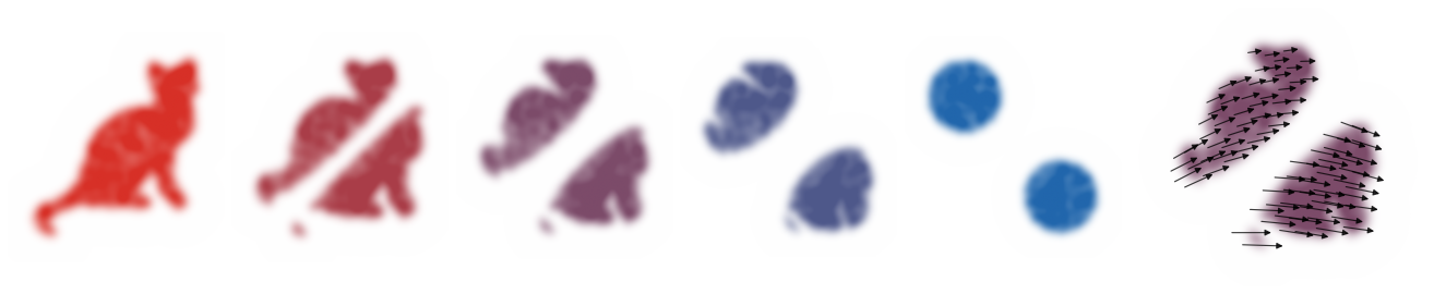
Benamou--Brenier geodesic between two sampled silhouettes. A discrete quadratic OT plan between finely subsampled cat and two-disks point clouds induces the McCann interpolation $Z_t=(1-t)X+tY$ , which is the Lagrangian realization of the least-action solution. The left panel renders local color images of the smaller-bandwidth kernel-smoothed densities with enough padding to include the full silhouettes. The right panel overlays shortened velocity arrows centered at evenly subsampled midpoint particles $Z_{1/2}$ ; each displayed arrow runs in data coordinates from a source-side tail to a target-side head along the matched characteristic direction $Y-X$ , but is not drawn as the full endpoint segment from $X$ to $Y$ .

The interactive demo keeps the same Lagrangian picture: particles are matched once, then move along straight characteristics. The time and velocity scale controls separate the path $\alpha_t$ from the underlying displacement field.

Interactive panel. Use the time and velocity-scale controls to follow the Benamou-Brenier geodesic as a moving density with an Eulerian velocity field.

Remark: Path-space formulation

Let $\Ss=C([0,1];\RR^d)$ be the space of continuous paths endowed with the uniform topology. For $t\in[0,1]$ define the evaluation map

P_t:\Ss\to\RR^d, \qquad P_t(\gamma)=\gamma(t).

(22)

The Benamou--Brenier cost admits the equivalent formulation

\Wass_2^2(\alpha_0,\alpha_1) = \inf_{M\in\Pp(\Ss)} \enscond{ \int_{\Ss}\!\int_0^1\norm{\dot\gamma(t)}^2\d t\,\d M(\gamma) }{ (P_0)_\sharp M=\alpha_0,\ (P_1)_\sharp M=\alpha_1 }.

(23)

If $\alpha_0$ has a density, the minimizer $M^*$ is unique. Its time marginals reproduce the optimal curve: $\alpha_t=(P_t)_\sharp M^*$ for all $t$ . Furthermore, for a.e. $t$ , denoting $Q_t(\gamma)=\dot\gamma(t)$ on absolutely continuous paths, the conditional law of the velocity is deterministic:

(P_t,Q_t)_\sharp M^*(\d x,\d q) = \alpha_t(\d x)\delta_{v_t^*(x)}(\d q),

(24)

where $v_t^*$ is the optimal velocity field in the Benamou--Brenier formulation. Hence $M^*$ concentrates on straight-line geodesics and, for a.e. $t$ , assigns exactly one direction at $\alpha_t$ -a.e. spatial point.

Extensions of the Dynamic Formulation¶

The same variational grammar extends beyond the quadratic Wasserstein distance. One changes either the kinetic exponent, the mobility or the balance equation, while keeping a continuity-type constraint and a convex perspective action.

Remark: Generalized Benamou--Brenier distances

The dynamic formulation is not specific to $\Wass_2$ . For measures with finite $p$ -th moments and $p>1$ , one has the analogous action formula

\Wass_p^p(\alpha_0,\alpha_1) = \inf_{\substack{\partial_t\alpha_t+\nabla\!\cdot(\alpha_t v_t)=0\\ \alpha_{t=0}=\alpha_0,\ \alpha_{t=1}=\alpha_1}} \int_0^1\!\int_{\RR^d} |v_t(x)|^p\,\d\alpha_t(x)\,\d t.

(25)

When $\alpha_t=\rho_t\,\d x$ and $m_t=\rho_t v_t$ , this becomes the convex perspective action

\int_0^1\!\int_{\RR^d} \frac{|m_t(x)|^p}{\rho_t(x)^{p-1}}\,\d x\,\d t, \qquad \partial_t\rho_t+\nabla\!\cdot m_t=0,

(26)

with the usual convention that the integrand is 0 if $(\rho,m)=(0,0)$ and $+\infty$ if $\rho=0$ but $m\neq0$ .

A second class of variants changes the mobility of the medium: the quadratic action $|m|^2/\rho$ is replaced by $|m|^2/\theta(\rho)$ for a suitable concave mobility $\theta$ . Under appropriate structural assumptions, this produces transport metrics adapted to nonlinear diffusions and finite-volume discretizations Dolbeault et al., 2009. On finite graphs and Markov chains, the analogous action uses an edge mobility, often the logarithmic mean of the endpoint densities, and leads to discrete Wasserstein geometries Maas, 2011Mielke, 2013. These extensions keep the same variational grammar as Benamou--Brenier: a continuity-type constraint, an action density, and geodesics obtained by minimizing an integrated kinetic cost.

Dynamic Unbalanced OT¶

Unbalanced dynamic transport is obtained by allowing mass to be created and destroyed along the path. The continuity equation is replaced by a balance equation, and the action penalizes both spatial motion and growth. This dynamic formulation underlies the Hellinger--Kantorovich and Wasserstein--Fisher--Rao metrics Liero et al., 2016Chizat et al., 2018; its equivalence with static entropy-transport and cone formulations is developed in Liero et al., 2018Chizat et al., 2018.

A representative quadratic action is

\partial_t\rho_t+\nabla\!\cdot m_t=s_t, \qquad \int_0^1\!\int \left( \frac{|m_t|^2}{\rho_t} +\kappa^2\frac{s_t^2}{\rho_t} \right)\d x\,\d t,

(27)

with the same perspective convention as above. Equivalently, writing $m_t=\rho_t v_t$ and $s_t=\rho_t g_t$ , one minimizes $\int_0^1\int(|v_t|^2+\kappa^2g_t^2)\d\rho_t\d t$ under

\partial_t\rho_t+\nabla\!\cdot(\rho_t v_t)=g_t\rho_t.

(28)

The parameter $\kappa$ fixes the relative cost of reaction and transport: changing it rescales the radial/angular balance in the associated cone metric. For measure-valued triples, the action is understood in the lower-semicontinuous perspective sense

\mathcal A_\kappa(\rho,m,s) \eqdef \int \left( \frac{\norm{\dot m}^2}{\dot\rho} + \kappa^2\frac{\dot s^2}{\dot\rho} \right)\d\lambda, \qquad (\dot\rho,\dot m,\dot s) = \left( \frac{\d\rho}{\d\lambda}, \frac{\d m}{\d\lambda}, \frac{\d s}{\d\lambda} \right),

(29)

where $\lambda$ dominates $\rho$ and the total variations of $m$ and $s$ . The value is independent of this choice. The convention is $0/0=0$ and $a/0=+\infty$ for $a>0$ , so finite action forces both the flux and the source to be absolutely continuous with respect to the transported mass.

Proposition: Static/Dynamic Equivalence for Unbalanced OT

Fix the action above and let $\mathcal C\mathcal W_\kappa$ be the cone value of the cone formulation of unbalanced OT, with the cone metric normalized to the same growth scale $\kappa$ . For nonnegative finite measures $\alpha_0,\alpha_1$ on $\RR^d$ , the dynamic value

\mathrm{WFR}_\kappa^2(\alpha_0,\alpha_1) \eqdef \inf_{\substack{\partial_t\rho_t+\nabla\cdot m_t=s_t\\ \rho_0=\alpha_0,\ \rho_1=\alpha_1}} \int_0^1 \mathcal A_\kappa(\rho_t,m_t,s_t)\,\d t

(30)

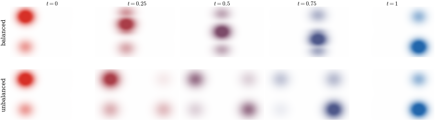
equals the static cone formulation $\mathcal C\mathcal W_\kappa(\alpha_0,\alpha_1)$ . Hence the static unbalanced problem and the balance-equation least-action problem define the same geodesic distance.

Balanced and unbalanced Sinkhorn-barycenter interpolations between two one-dimensional Gaussian mixtures with swapped modal masses. The balanced row conserves total mass, so excess mass from the dominant left mode must move along the line toward the dominant right target mode, producing transient mass in the middle. The unbalanced row uses KL-relaxed marginal constraints; mass can be attenuated near overrepresented modes and recreated near underrepresented modes, giving a reaction--transport interpolation closer to the Wasserstein--Fisher--Rao intuition.

The interactive demo below exposes this balance directly. A high reaction weight keeps more mass local by fading and recreating modes, while the balanced path must carry mass through space.

Interactive panel. Use the growth and time controls to compare motion with source terms in dynamic unbalanced transport.

Algorithm: Douglas--Rachford for dynamic Benamou--Brenier

Input: Functionals $\mathcal F,\mathcal G=\iota_{\mathcal C}$ , proximal parameter $\tau>0$ , initial field $Z^0$ .

Output: Discrete density-momentum field $U^\star$ .

For $k=0,1,\ldots$ do:

$U^{k+1}=\prox_{\tau\mathcal F}(Z^k).$
Project reflected point: $\widetilde U^{k+1} = \prox_{\tau\mathcal G}(2U^{k+1}-Z^k) = \Proj_{\mathcal C}(2U^{k+1}-Z^k).$
Update $Z^{k+1}=Z^k+\widetilde U^{k+1}-U^{k+1}.$
If $\norm{U^{k+1}-\widetilde U^{k+1}}\leq\mathrm{tol}$ then:

Return $U^{k+1}$ .

References¶

Dacorogna, B., & Moser, J. (1990). On a Partial Differential Equation Involving the Jacobian Determinant. Annales de l’Institut Henri Poincaré C, Analyse Non Linéaire, 7(1), 1–26.
Benamou, J.-D., & Brenier, Y. (2000). A computational fluid mechanics solution to the Monge-Kantorovich mass transfer problem. Numerische Mathematik, 84(3), 375–393.
Dolbeault, J., Nazaret, B., & Savaré, G. (2009). A new class of transport distances between measures. Calculus of Variations and Partial Differential Equations, 34(2), 193–231.
Maas, J. (2011). Gradient flows of the entropy for finite Markov chains. Journal of Functional Analysis, 261(8), 2250–2292.
Mielke, A. (2013). Geodesic convexity of the relative entropy in reversible Markov chains. Calculus of Variations and Partial Differential Equations, 48(1–2), 1–31.
Liero, M., Mielke, A., & Savaré, G. (2016). Optimal transport in competition with reaction: the Hellinger–Kantorovich distance and geodesic curves. SIAM Journal on Mathematical Analysis, 48(4), 2869–2911.
Chizat, L., Schmitzer, B., Peyré, G., & Vialard, F.-X. (2018). An interpolating distance between optimal transport and Fisher–Rao metrics. Foundations of Computational Mathematics, 18(1), 1–44.
Liero, M., Mielke, A., & Savaré, G. (2018). Optimal entropy-transport problems and a new Hellinger–Kantorovich distance between positive measures. Inventiones Mathematicae, 211(3), 969–1117.
Chizat, L., Peyré, G., Schmitzer, B., & Vialard, F.-X. (2018). Unbalanced optimal transport: dynamic and Kantorovich formulation. Journal of Functional Analysis, 274(11), 3090–3123.