Semi-discrete and Wasserstein-1

This chapter focuses on two computationally useful degeneracies of the dual problem. Semi-discrete optimal transport turns a continuous-to-discrete map into finite-dimensional geometry, while $\Wass_1$ replaces convex potentials by Lipschitz functions and flow fields. The material connects computational geometry Aurenhammer et al., 1998Mérigot, 2011Mérigot, 2013 with the Kantorovich--Rubinstein and Beckmann formulations Kantorovich & Rubinstein, 1958Beckmann, 1952.

from pathlib import Path
import sys

from IPython.display import Image as DisplayImage
from IPython.display import display

here = Path.cwd()
myst_dir = None
for candidate in [here, here.parent, here / "myst", here.parent / "myst", here.parent.parent / "myst"]:
    if (candidate / "ot4ml_web.py").exists():
        myst_dir = candidate.resolve()
        sys.path.insert(0, str(myst_dir))
        break

if myst_dir is None:
    raise RuntimeError("Could not locate myst/ot4ml_web.py")

repo_root = myst_dir.parent
thumbnails = repo_root / "notebooks-figures" / "thumbnails"

def show_book_figure(name, width=760):
    display(DisplayImage(filename=str(thumbnails / f"{name}.png"), width=width))

Semi-dual¶

The semi-dual eliminates one potential by an exact $c$-transform. It keeps concavity while removing explicit inequality constraints.

Write the dual problem as

where $\mathcal{E}(f,g)$ is the dual objective, with value $-\infty$ when the feasibility constraint fails. Optimizing out $g$ exactly gives the semi-dual problem

Partial maximization of a concave problem preserves concavity, so $\widetilde{\mathcal{E}}$ is still concave. The advantage is that the explicit inequality constraint has disappeared, which allows simpler optimization algorithms.

Semi-discrete¶

The semi-discrete case is the setting where dual potentials become weights of Laguerre cells. This gives both geometry and algorithms for quantization and density fitting.

Discrete Targets and Laguerre Cells¶

Consider the case where

is discrete. The same construction applies if $\alpha$ is discrete, after exchanging the roles of $\alpha$ and $\beta$. For a dual vector $g\in\RR^m$, the discrete $\bar c$-transform is

This maps a vector $g$ to a continuous function under the same regularity assumptions on $c$ as in the continuous setting. It coincides with the usual $c$-transform when the target space is restricted to the support of $\beta$. Using this transform when $\beta$ is discrete yields the finite-dimensional semi-dual

The geometric object encoded by the dual weights is a weighted nearest-neighbor diagram: each source point is assigned to the target atom that realizes the discrete $\bar c$-transform.

For quadratic costs, varying the dual weights moves the walls between adjacent cells while keeping them parallel. This is the geometric mechanism by which the cell masses are adjusted.

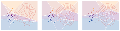
show_book_figure("semidiscrete-laguerre-cells")

Laguerre cells for semi-discrete quadratic transport. The red contours show a continuous source density $\alpha$ given by a three-component Gaussian mixture on the right. The twenty-one colored circular sites are the atoms of the discrete target $\beta$, sampled from a compact cloud on the left; each site color matches its Laguerre cell. Starting from ordinary Voronoi cells, semi-dual weight updates deform the cells so that the $\alpha$-mass captured by each cell approaches the prescribed target mass.

The interactive demo exposes the dual-weight mechanism directly. Increase the number of weight updates to watch cells with too little mass expand and cells with too much mass shrink.

Mass Balance¶

The semi-dual energy can be rewritten as

The first-order optimality condition says that solving the semi-discrete dual amounts to choosing weights $g$ so that

At optimality, the transport map is piecewise constant: it sends $x\in\mathcal{L}_j(g)$ to $y_j$. For the quadratic cost, uniqueness follows from Brenier’s theorem when $\alpha$ has a density.

Quadratic power diagrams have polyhedral cells and can be computed efficiently using computational-geometry algorithms Aurenhammer, 1987Aurenhammer et al., 1998Mérigot, 2011. One classical construction lifts sites to $(y_j,\norm{y_j}^2-g_j)\in\RR^{d+1}$ and obtains the power diagram by projecting the lower envelope of their convex hull. In dimensions two and three, Chan’s output-sensitive convex-hull algorithm has complexity $O(m\log Q)$ for $m$ sites and $Q$ hull vertices Chan, 1996.

Stochastic Optimization¶

The semi-discrete formulation is useful because the objective is an expectation with respect to $\alpha$:

Away from cell boundaries, the stochastic gradient of the integrand is

an unbiased estimator of $\nabla\mathcal{E}(g)$ when cell boundaries have $\alpha$-measure zero. One can therefore maximize the semi-dual without first discretizing $\alpha$: the measure is used as a black box from which independent samples are drawn, a natural setup in high-dimensional statistics and machine learning.

Starting from $g^{(0)}=0$, stochastic gradient ascent draws $x_\ell\sim\alpha$ and performs

The step size must decay so that sampling noise averages out. A typical schedule is

Under standard stochastic-approximation assumptions,

where $g^\star$ is a maximizer and the expectation is over the i.i.d. samples. This stochastic viewpoint is one of the main algorithmic advantages of the semi-discrete formulation Mérigot, 2011Genevay et al., 2016.

Optimal Quantization¶

Optimal quantization asks for the best discrete approximation of a measure by $m$ codepoints. It is the geometric core of vector quantization, compression and $k$-means clustering.

For a measure $\alpha$, define

This problem is classical in approximation theory and information theory Graf & Luschgy, 2000Lloyd, 1982. The optimal-transport formulation emphasizes that one optimizes both the support locations $Y$ and, unless prescribed, the masses $b$.

This deterministic rate mirrors the empirical optimal-transport sample-complexity rate: both are governed by the spacing $m^{-1/d}$ of points in dimension $d$. Quantization is best-case and deterministic, while empirical OT is random, but both display the same curse of dimensionality.

For fixed codepoints $Y$, the problem is convex with respect to the weights $b$. The dependence on $Y$ is nonconvex and is generally computationally hard. In one dimension, monotonicity fixes the ordering of cells, reducing the problem to interval endpoints and centroids; for the uniform law with the quadratic cost, the optimal centroids are equally spaced.

Consequently, the quantization energy can be written in nearest-centroid form:

At a differentiability point of this energy, each local minimizer satisfies the centroid condition

For the squared Euclidean cost, this becomes

Lloyd’s algorithm, also known as the $k$-means algorithm, iterates this fixed point: assign points to nearest sites, then replace each site by the centroid of its cell Lloyd, 1982. With standard tie-breaking, the objective decreases at each step. Since the problem is nonconvex in $Y$, the iterates generally converge only to a local minimum. Good seeding matters; for squared Euclidean costs, $k$-means++ gives a logarithmic approximation guarantee in expectation Arthur & Vassilvitskii, 2007.

show_book_figure("semidiscrete-lloyd-quantization")

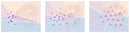
Lloyd quantization for the same continuous density and twenty-one initial sites as the Laguerre-cell figure. The red contours show the density $\alpha$, while the colored disks are the current codepoints and have the same colors as their Voronoi cells. The iterations move the initially left-located sites toward the high-density region and reshape the cells according to centroidal Voronoi geometry.

The interactive demo separates the nonconvex geometry from the fixed-point update: increase the iteration counter and watch sites migrate toward the density before settling into a local centroidal configuration.

Wasserstein-1 Norm¶

The $\Wass_1$ distance has an especially transparent dual: the admissible potentials are exactly 1-Lipschitz test functions. This makes $\Wass_1$ the meeting point between transport, PDE formulations and weak norms on signed measures.

c-Transform for Wasserstein-1¶

Assume that $d$ is a distance on $\X=\Y$ and take the ground cost $c(x,y)=d(x,y)$.

Using the alternating $c$-transform scheme from the dual chapter, one can replace the dual pair by $(f,-f)$ with $\Lip(f)\le1$. The Kantorovich dual therefore becomes the Kantorovich--Rubinstein formula

This expression depends only on the signed measure $\alpha-\beta$. It therefore extends to finite signed measures of total mass zero and defines the Kantorovich--Rubinstein norm on that space Kantorovich & Rubinstein, 1958.

For a discrete signed measure $\alpha-\beta=\sum_k r_k\delta_{z_k}$ with $\sum_k r_k=0$,

This finite-dimensional linear program can be solved by generic interior-point or first-order methods; structured graph versions admit the flow formulations described below.

When $d(x,y)=|x-y|$ on $\RR$, ordering the support points $z_1\le z_2\le\cdots$ reduces the constraints to neighboring pairs:

In one dimension this is equivalent to the closed-form cumulative formula introduced earlier.

Wasserstein-1 on Euclidean Spaces¶

For $\X=\Y=\RR^d$ with $c(x,y)=\norm{x-y}$, the global Lipschitz constraint in the Kantorovich--Rubinstein formula can be made local as a uniform bound on the gradient:

Dualizing this expression with respect to vector fields $m:\RR^d\to\RR^d$ gives the fixed-divergence problem

often called the Beckmann formulation Beckmann, 1952. The vector field $m(x)$ describes local movement of mass. Outside the support of the two input measures, $\operatorname{div}(m)=0$, which is conservation of mass.

Once discretized with finite elements, the dual Lipschitz problem and the Beckmann problem become nonsmooth convex optimization problems. The same formulation extends to Riemannian manifolds by replacing the Euclidean distance by geodesic distance and interpreting gradient and divergence as differential operators on the manifold.

This graph distance turns $\Wass_1$ into a finite-dimensional flow problem.

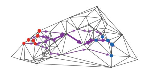
show_book_figure("w1-graph-transport-flow")

Graph Beckmann formulation of $\Wass_1$ on a Delaunay graph. Red and blue disks encode the positive and negative parts of $r=\alpha-\beta$. Violet arrows display the signed edge flow $m$: orientation gives the sign, width is proportional to $\sqrt{|m_e|}$, and the flow satisfies the conservation constraint $\operatorname{div}_G m=r$.

The interactive graph view lets the source and sink clusters move and changes the graph resolution. It makes the transshipment interpretation of $\Wass_1$ visible: signed mass is routed through local edges rather than matched only by straight source-to-target segments.

This graph formulation is the transshipment version of $\Wass_1$. It is the natural discrete analogue of the Beckmann formulation: gradients are edge differences, divergences are incidence-matrix balances, and geodesic distance is shortest-path length. It can be solved by min-cost flow methods on sparse graphs, while entropic or KL-projection variants lead to flow-Sinkhorn algorithms for graph $\Wass_1$ Beckmann, 1952Peyré, 2026.