Monge Problem between Measures

The goal of this chapter is to pass from finite matching to transport between arbitrary probability laws. The central stakes are to define measures, push-forwards and Monge maps carefully enough that the discrete picture survives, while exposing why deterministic maps can fail to exist. Monge’s original formulation Monge, 1781 and modern treatments Villani, 2003Villani, 2009Santambrogio, 2015Rachev & Rüschendorf, 1998 are the conceptual background for this transition.

The previous chapter handled two sets with the same number of points. To relax this to a more general setting, one needs probability distributions, so that points may carry unequal masses and continuous densities can be treated in the same language as finite clouds.

from pathlib import Path
import sys

from IPython.display import Image as DisplayImage
from IPython.display import display

here = Path.cwd()
myst_dir = None
for candidate in [here, here.parent, here / "myst", here.parent / "myst", here.parent.parent / "myst"]:
    if (candidate / "ot4ml_web.py").exists():
        myst_dir = candidate.resolve()
        sys.path.insert(0, str(myst_dir))
        break

if myst_dir is None:
    raise RuntimeError("Could not locate myst/ot4ml_web.py")

repo_root = myst_dir.parent
thumbnails = repo_root / "notebooks-figures" / "thumbnails"

def show_book_figure(name, width=760):
    display(DisplayImage(filename=str(thumbnails / f"{name}.png"), width=width))

Measures¶

Measures are the language that lets point clouds, densities and singular objects be handled uniformly. We only recall the facts needed later: integration, total variation, densities and probabilistic laws.

Histograms¶

Discrete And Empirical Measures¶

The Dirac mass should be thought of as a unit of mass infinitely concentrated at one location.

An empirical probability distribution is uniform on a point cloud,

\al=\frac1n\sum_{i=1}^n\delta_{x_i}.

(3)

In applications, it is useful to manipulate both the positions $x_i$ and the weights $a_i$ . Moving the positions is a Lagrangian discretization; changing the weights is an Eulerian one. The Lagrangian view is often more adaptive, but it tends to break convexity.

General Measures¶

We consider Borel measures $\al\in\Mm(\X)$ on a metric space $(\Xx,d)$ . This means that $\al(A)$ is defined for every Borel set $A$ , obtained from open sets by countable unions, intersections and complements. Unless otherwise stated, the measures are finite.

A Dirac measure is defined by $\delta_x(A)=1$ if $x\in A$ and 0 otherwise. For the discrete measure above,

\al(A)=\sum_{x_i\in A} a_i .

(4)

We denote by $\Mm_+(\X)$ the set of positive finite measures on $\X$ and by $\Mm_+^1(\X)$ the set of probability measures, i.e. positive measures of total mass one.

Polish Metric Spaces¶

Many measure-theoretic statements used later require a mild regularity assumption on the underlying space. The point is not to restrict applications, since Euclidean spaces, complete separable manifolds and separable Hilbert spaces are covered, but to exclude pathological measurable spaces where disintegration, tightness or weak convergence can fail to behave properly.

Polish spaces are the natural ambient category for probability measures. Borel probability measures on them are regular, tightness gives compactness criteria, regular conditional probabilities and disintegrations exist under standard assumptions, and Wasserstein spaces remain Polish; see Proposition Proposition: Wasserstein Spaces As Ground Spaces.

Radon Measures¶

Using Lebesgue integration, a Borel measure computes integrals of measurable functions. We write the duality pairing as

\langle f,\al\rangle \eqdef \int f(x)\d\al(x).

(5)

For a discrete measure this becomes

\int_\X f(x)\d\al(x)=\sum_{i=1}^n a_i f(x_i).

(6)

Integration against a finite measure on a compact space defines a continuous linear form on the Banach space $(\Cc(\Xx),\|\cdot\|_\infty)$ , since $|\int f\d\al|\leq \|f\|_\infty |\al|(\Xx)$ . Conversely, the Riesz--Markov--Kakutani representation theorem identifies every continuous linear form on $\Cc(\Xx)$ with integration against a finite signed Radon measure Rudin, 1987Bogachev, 2007. This is the duality $\Mm(\Xx)=\Cc(\Xx)^*$ that later supports convex duality.

Relative Densities¶

On $\RR^d$ the reference $\lambda$ is often Lebesgue measure $\d x$ .

Total Variation¶

The norm inherited from the duality $\Mm(\Xx)=\Cc(\Xx)^*$ is the total variation norm.

The absolute value of a signed measure is

|\al|(A) \eqdef \sup_{A=\cup_i B_i}\sum_i |\al(B_i)|,

(10)

where the supremum is over finite or countable measurable partitions of $A$ . If $\al=\sum_i a_i\delta_{x_i}$ with distinct atoms, then $|\al|=\sum_i |a_i|\delta_{x_i}$ . If $\d\al(x)=\rho(x)\d\lambda(x)$ , then $\d|\al|(x)=|\rho(x)|\d\lambda(x)$ .

For absolutely continuous measures $\d\al=\rho_\al\d\lambda$ and $\d\be=\rho_\be\d\lambda$ ,

\|\al-\be\|_{\TV} = \int_\Xx |\rho_\al(x)-\rho_\be(x)|\d\lambda(x).

(13)

For two discrete measures written on the same union of supports, $\al=\sum_k a_k\delta_{z_k}$ and $\be=\sum_k b_k\delta_{z_k}$ , with missing coefficients set to zero,

\|\al-\be\|_{\TV}=\sum_k |a_k-b_k|.

(14)

Probabilistic Interpretation¶

Radon probability measures represent laws of random variables. A random variable with values in $\X$ is a measurable map $X:\Omega\to\X$ from an abstract probability space $(\Omega,\PP)$ . Its law is the Radon probability measure $\al$ defined by

\al(A)=\PP\{\omega\in\Omega : X(\omega)\in A\}.

(15)

Integrals with respect to the law are expectations:

\int_\X f(x)\d\al(x)=\mathbb{E}[f(X)].

(16)

Push Forward¶

Push-forwards encode how maps move mass. This short section is the bridge between deterministic maps and linear operations on measures.

For a continuous map $\T:\X\to\Y$ , the push-forward operator $\T_\sharp:\Mm(\X)\to\Mm(\Y)$ sends a Dirac mass to $\T_\sharp\delta_x=\delta_{\T(x)}$ . For discrete measures,

\T_\sharp\al=\sum_i a_i\delta_{\T(x_i)}.

(17)

Moving from $\T$ to $\T_\sharp$ linearizes the action of a map at the price of moving from the space $\Xx$ to the measure space $\Mm(\Xx)$ .

Remark: Pullback and push-forward

If $\T:\X\to\Y$ is continuous, the pullback by $\T$ is the linear operator

\T^\sharp:\Cc(\Y)\to\Cc(\X), \qquad \T^\sharp g=g\circ\T .

(20)

The definition of the push-forward is exactly the dual relation between this pullback on functions and the action of $\T_\sharp$ on measures:

\int_\X \T^\sharp g(x)\d\mu(x) = \int_\Y g(y)\d(\T_\sharp\mu)(y).

(21)

In pairing notation,

\left\langle \T^\sharp g,\mu\right\rangle_{\Cc(\X),\Mm(\X)} = \left\langle g,\T_\sharp\mu\right\rangle_{\Cc(\Y),\Mm(\Y)}.

(22)

Thus push-forward is the adjoint operation to pullback, with the direction reversed. The two arrows should not be confused: $\T_\sharp$ transports mass from $\X$ to $\Y$ , whereas $\T^\sharp$ transports test functions from $\Y$ back to $\X$ .

Monge’s Formulation¶

Monge’s problem asks for a deterministic map transporting one law onto another while minimizing a prescribed cost. It is geometrically direct, because every source point is assigned one destination, but analytically fragile: the feasible set is non-convex, it can be empty, and a map cannot split mass. These limitations motivate Kantorovich’s relaxation in the next chapter.

Monge Problem¶

Given $\al\in\Mm_+^1(\Xx)$ , $\be\in\Mm_+^1(\Yy)$ and a cost $c:\Xx\times\Yy\to\RR_+$ , the Monge problem is

\Monge_c(\al,\be) \eqdef \inf_{\T:\Xx\to\Yy} \left\{ \int_\Xx c(x,\T(x))\d\al(x) \;:\; \T_\sharp\al=\be \right\}.

(26)

The constraint $\T_\sharp\al=\be$ means that $\T$ pushes the mass of $\al$ onto $\be$ .

Proposition: Empirical Monge Maps And Matchings

Assume that the source atoms $x_1,\ldots,x_n$ are distinct and

\al=\frac1n\sum_{i=1}^n\delta_{x_i}, \qquad \be=\frac1n\sum_{j=1}^n\delta_{y_j}.

(27)

If $\T_\sharp\al=\be$ , then for each distinct target value $z$ in the support of $\be$ , exactly $n\be(\{z\})$ source atoms are mapped to $z$ . In particular, if the $y_j$ are distinct, then there is a permutation $\sigma\in\Perm(n)$ such that $\T(x_i)=y_{\sigma(i)}$ .

Conversely, every assignment of source atoms to target atoms with the correct masses defines a feasible Monge map on the support of $\al$ , and in the distinct-target case

\int_\Xx c(x,\T(x))\d\al(x) = \frac1n\sum_{i=1}^n c(x_i,y_{\sigma(i)}).

(28)

If source locations are repeated, they should first be merged into atoms with larger masses; such atoms cannot be split by a Monge map.

Example: Semi-discrete Monge maps

The Monge formulation is not symmetric in $\al$ and $\be$ . It makes sense, for instance, when $\al$ has a density with respect to Lebesgue measure and $\be$ is discrete. On $\Xx=\Yy=\RR^d$ , let $\be=\sum_j b_j\delta_{y_j}$ be supported on $\{y_1,\ldots,y_m\}$ . A map $\T$ such that $\T_\sharp\al=\be$ defines a segmentation of the space into cells

C_j\eqdef \T^{-1}(y_j), \qquad \al(C_j)=b_j.

(30)

This is the semi-discrete setting. Chapter Paragraph explains how the cells become Laguerre cells for prescribed masses and ordinary Voronoi cells when the masses are free. If one exchanges the roles of $\al$ and $\be$ so that $\al$ is discrete, then no valid $\T$ exists in general: it is not possible to push forward a discrete measure to a measure with density.

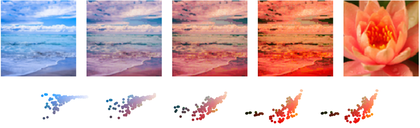
The next figure shows a finite-dimensional instance of this deterministic viewpoint. The source and target measures are empirical color clouds in RGB space, and the map transports colors while leaving pixel positions fixed. Grayscale equalization is one-dimensional, but full palette transfer requires transporting empirical measures in a three-dimensional color space. Early methods used affine statistics or iterated one-dimensional projections Reinhard et al., 2001Pitié et al., 2005; replacing these projections by a three-dimensional OT map gives a more intrinsic palette match Rabin et al., 2011.

Color transfer as a Monge map in RGB space, from a beach photograph to a flower photograph. The top row applies the palette map to the source image; the bottom row shows the empirical color clouds in the RGB cube. Only colors are transported here, not pixel locations.

Interactive panel. Use the interpolation, resolution, target palette, and contrast controls to replay the RGB color transport while keeping pixel locations fixed.

Monge Distance¶

When $\Xx=\Yy$ and $c(x,y)=d(x,y)^p$ for a metric $d$ , set

\mathcal{E}_\al(\T) \eqdef \int_\Xx d(x,\T(x))^p\d\al(x).

(31)

The Monge value defines the directed quantity

\widetilde{\Wass}_p(\al,\be)^p \eqdef \inf_{\T:\Xx\to\Xx} \left\{ \mathcal{E}_\al(\T) \;:\; \T_\sharp\al=\be \right\}.

(32)

If the constraint set is empty, then $\widetilde{\Wass}_p(\al,\be)=+\infty$ .

The directed value $\widetilde{\Wass}_p$ is useful conceptually, but it is too rigid to be the main distance between measures: it can be infinite and asymmetric. Kantorovich’s formulation remedies both issues by replacing maps with couplings.

Existence And Uniqueness Of The Monge Map¶

This section records the main regimes where Monge’s deterministic formulation becomes well posed. Brenier’s theorem is the central result: for the squared Euclidean cost, absolute continuity of the source restores existence, uniqueness and convex-potential structure.

Brenier’s Theorem¶

Brenier’s theorem Brenier, 1987Brenier, 1991 ensures that in $\RR^d$ , for the quadratic cost, absolute continuity of the source is enough for Monge’s problem to have a unique solution. It also gives the decisive structural description: the optimal map is the gradient of a convex potential.

Remark: Beyond the quadratic Euclidean cost

Brenier’s theorem is the cleanest statement because the squared Euclidean cost turns optimal maps into gradients of convex functions. For costs $c(x,y)=\norm{x-y}^p$ with $p>1$ , or more generally costs $c(x,y)=h(x-y)$ with $h$ smooth and strictly convex, the same strategy gives a unique optimal map under absolute continuity of the source, but the map is written in terms of a $c$ -convex potential. On a Riemannian manifold, the local analogue for the cost $d_M(x,y)^2/2$ uses the exponential map

\T(x)=\exp_x(-\nabla\phi(x)),

(36)

where $\phi$ is $c$ -convex. The main additional issues are the cut locus and regularity of geodesics, which is why the Euclidean statement is usually presented first. These extensions are part of McCann’s displacement convexity theory and the general theory of optimal maps on manifolds McCann, 1997Villani, 2009.

Brenier’s theorem should be read through the analogy between convex gradients and increasing functions. The gradient of a convex function is a monotone field:

\langle \nabla\phi(x)-\nabla\phi(x'),x-x'\rangle\geq0.

(37)

Remark: Monotone fields need not be gradients

In dimensions larger than one, not all monotone fields are gradients of convex functions. Consider in $\RR^2$ the rotation matrix

R_\theta=\begin{pmatrix} \cos\theta & -\sin\theta\\ \sin\theta & \cos\theta \end{pmatrix}.

(38)

The linear map $x\mapsto R_\theta x$ is monotone as soon as $|\theta|\leq\pi/2$ , because

\dotp{R_\theta x-R_\theta x'}{x-x'} = \dotp{R_\theta(x-x')}{x-x'} = \cos(\theta)\norm{x-x'}^2\geq0.

(39)

However, for $\theta\neq0$ , $R_\theta$ is not symmetric and therefore cannot be the gradient of a scalar potential. Indeed, if a linear field $Ax$ equals $\nabla\phi(x)$ , then its Jacobian $A$ must be symmetric; equivalently, a quadratic potential $\phi(x)=\dotp{Bx}{x}/2$ has gradient $((B+B^\top)/2)x$ . Thus monotonicity is weaker than Brenier optimality in dimension $d\geq2$ .

Polar Factorization¶

Brenier’s theorem provides a canonical way to extract the monotone part of an arbitrary map. Suppose one starts from a square-integrable deformation $u:\Omega\to\RR^d$ . Its law $\nu=u_\sharp\lambda$ records where the mass ends up, but forgets how the points of $\Omega$ were labelled. Brenier’s polar factorization Brenier, 1987Brenier, 1991 separates these effects: a measure-preserving rearrangement $s$ changes labels without changing mass, then the unique convex-gradient map $\nabla\phi$ sends the uniform source to the output law.

For linear maps under a Gaussian reference, this reduces to the usual matrix polar decomposition. If $X\sim\Gaussian(0,\Id)$ and $u(x)=Ax$ , then $u_\sharp\Gaussian(0,\Id)=\Gaussian(0,AA^\top)$ . The Brenier map from $\Gaussian(0,\Id)$ to this Gaussian is $x\mapsto Sx$ , where $S=(AA^\top)^{1/2}$ is symmetric positive semidefinite. Hence

A=SO, \qquad O=S^\dagger A.

(41)

The factor $Sx$ is the convex-gradient transport part, while $Ox$ preserves the standard Gaussian law.

Displacement Interpolation¶

An optimal map does not only match two endpoint measures; it tells how to draw a path between them. Each particle keeps its identity and travels at constant speed from its initial position to its image.

Proposition: Directed Monge Displacement Geodesics

Let $p\geq1$ , let $\al,\be\in\Mm_+^1(\RR^d)$ have finite $p$ -th moments, and let $\T$ be an optimal map for $\widetilde{\Wass}_p(\al,\be)$ . Set $\al_t=(\T_t)_\sharp\al$ with $\T_t=(1-t)\Id+t\T$ . Assume that, for every $t<1$ , $\T_t$ is one-to-one on a full $\al$ -measure Borel set. Then, for $0\leq s\leq t\leq1$ ,

\widetilde{\Wass}_p(\al_s,\al_t) = (t-s)\widetilde{\Wass}_p(\al,\be).

(43)

Thus $t\mapsto\al_t$ is an oriented constant-speed geodesic for the directed Monge distance. For $p=2$ , this applies to the Brenier map under the hypotheses of Brenier’s theorem.

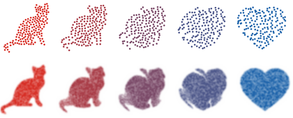
McCann displacement interpolation between a cat silhouette and a heart silhouette. The first row displays a small farthest-point subset of transported particles along $T_t(x)=(1-t)x+tT(x)$ . The second row renders kernel-smoothed densities from a denser transported cloud as color images: white means zero density, while high density saturates in the red-to-blue interpolation color of the corresponding time.

Interactive panel. Use the interpolation and particle controls to compare the particle motion with the evolving density during McCann displacement interpolation.

Regularity And The Monge-Ampere Equation¶

The previous results identify the optimal map. Regularity theory asks when this map is a classical smooth deformation rather than only an almost-everywhere gradient. For quadratic costs this becomes the regularity theory of the Monge--Ampere equation.

Remark: Regularity, weak maps, and splitting

Caffarelli’s theorem should be read as a warning as well as a theorem. Brenier’s theorem gives existence and uniqueness under mild assumptions, but smoothness requires density bounds, smoothness and convex geometry that are rarely satisfied by empirical, manifold-supported or neural generative distributions. In such applications, the exact OT map is often only weakly defined, possibly unstable, and better represented by a coupling, an entropic approximation or a learned parametric surrogate.

Even without smoothness, the convex potential is locally Lipschitz on the interior of its domain, so $\nabla\phi$ is defined Lebesgue-almost everywhere. If the source measure does not satisfy the non-splitting hypotheses of Brenier’s theorem, the correct relaxed object is instead an optimal Kantorovich plan concentrated on the graph of the set-valued map $\partial\phi$ . At points where $\partial\phi(x)$ contains several target locations, the plan may split the mass starting from $x$ . Thus the subdifferential still describes the geometry of optimality, but the transport object is a coupling rather than a single-valued map.

For smooth densities, the change-of-variables formula gives the Monge--Ampere equation

\det(\nabla^2\phi(x))\density{\be}(\nabla\phi(x)) = \density{\al}(x).

(46)

With suitable boundary conditions, this characterizes the Brenier potential up to an additive constant among convex solutions. The following proposition records the infinitesimal form.

One-Dimensional Transport And Quantiles¶

In one dimension, optimal transport is completely explicit. The cumulative distribution function orders the mass, and the optimal coupling is obtained by matching equal quantile levels. This case is both a computational tool and the template for several linearized constructions used later.

If $\al$ has no atoms, the map

\T=\cumul{\be}^{-1}\circ\cumul{\al}

(54)

satisfies $\T_\sharp\al=\be$ . For the cost $c(x,y)=|x-y|^2$ , this map is nondecreasing and therefore the derivative of a convex function in dimension one.

The quantile formula above means that $\al\mapsto\cumul{\al}^{-1}$ embeds one-dimensional Wasserstein geometry isometrically into a linear $L^p$ space. For $p=2$ , Wasserstein geometry on probability measures over the real line is Hilbertian.

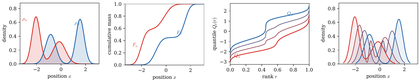
One-dimensional transport through quantiles. The same two smooth laws are shown as densities, cumulative functions and quantile functions. The last panel displays the displacement interpolation obtained by the linear quantile path $Q_t=(1-t)Q_\alpha+tQ_\beta$ , which is the explicit one-dimensional $\Wass_2$ geodesic.

Interactive panel. Use the time and endpoint controls to follow the one-dimensional Wasserstein geodesic through quantiles, CDFs, and densities.

In quantile coordinates, the interpolating measure is characterized by

\cumul{\al_t}^{-1}(r) = (1-t)\cumul{\al}^{-1}(r)+t\cumul{\be}^{-1}(r), \qquad r\in(0,1).

(61)

For $p=1$ , the cumulative formula above shows that $\Wass_1$ is a norm on signed measures with zero total mass once they are identified with their cumulative primitives.

Triangular Rearrangements¶

There is another canonical way to build transport maps in several dimensions: transport one coordinate at a time by conditional one-dimensional quantiles. This construction is not usually cost-optimal, but it gives a deterministic rearrangement under weak assumptions.

Triangular rearrangement between the same cat and heart densities as in the McCann interpolation figure. The panels are computed directly on image histograms. The first three transitions move mass horizontally by the monotone rearrangement between the $x$ -marginals; the pivot has the target horizontal marginal. The last three transitions keep each column fixed and move mass vertically by one-dimensional monotone rearrangements between conditional laws.

Interactive panel. Use the horizontal and vertical interpolation sliders to inspect the Knothe triangular rearrangement one coordinate update at a time.

This construction transports successively along coordinate axes and is often called axis-wise transport. It depends on the chosen ordering of coordinates and is not generally optimal for the quadratic cost. It is nevertheless a useful limiting object: Brenier maps for increasingly anisotropic quadratic costs converge to triangular rearrangements under suitable assumptions Carlier et al., 2010.

Proposition: Anisotropic Brenier Maps Converge To Knothe--Rosenblatt

Let $\alpha,\beta$ be compactly supported probability measures on $\RR^d$ with densities bounded above and below on rectangular supports, and assume that the conditional laws entering the triangular rearrangement are atomless. For $\epsilon>0$ , set

c_\epsilon(x,y) \eqdef \sum_{k=1}^d \epsilon^{k-1}|x_k-y_k|^2 .

(63)

Let $T_\epsilon$ be the Monge map from $\alpha$ to $\beta$ for $c_\epsilon$ , and let $T_{\mathrm{KR}}$ be the triangular Knothe--Rosenblatt rearrangement with the same coordinate order. Then

T_\epsilon \longrightarrow T_{\mathrm{KR}} \qquad\text{in }L^2(\alpha;\RR^d) \qquad\text{as }\epsilon\to0 .

(64)

Example: Linear obstruction to composing Brenier maps

In higher dimension, Brenier maps for the quadratic cost are gradients of convex functions, and such maps do not generally remain gradients after composition. The simplest obstruction is linear. If $\T_1(x)=A_1x$ and $\T_2(x)=A_2x$ with $A_1,A_2$ symmetric positive definite, then $\T_2\circ\T_1$ has matrix $A_2A_1$ . It is a gradient field only when this product is symmetric, equivalently $A_1A_2=A_2A_1$ . Gaussian transport gives a concrete instance: between nondegenerate Gaussian laws, the Brenier map is affine with symmetric positive definite linear part. Compositions of Gaussian optimal maps are therefore optimal only in special commuting situations, for instance when all covariance matrices are simultaneously diagonalizable. Otherwise the composition contains a rotational or shearing component and is not the Brenier map between the initial and final Gaussians.

Algorithm: Quantile rearrangement and one-dimensional geodesic

Input: One-dimensional probability measures $\alpha,\beta$ ; time $t\in[0,1]$ .

Output: Quantile coupling, Monge map when defined, and geodesic point $\alpha_t$ .

Compute $\cumul{\al}$ , $\cumul{\be}$ and generalized inverses.

Couple equal quantile levels: $X=\cumul{\al}^{-1}(r), \qquad Y=\cumul{\be}^{-1}(r), \qquad r\in(0,1).$

If $\alpha$ has no atoms then:

Set $T(x)=\cumul{\be}^{-1}(\cumul{\al}(x)).$

Interpolate quantiles: $Q_t(r)=(1-t)\cumul{\al}^{-1}(r)+t\cumul{\be}^{-1}(r), \qquad \al_t=(Q_t)_\sharp\mathrm{Leb}_{[0,1]}.$ Return $(X,Y)$ , $T$ if defined, and $\alpha_t$ .

Algorithm: Knothe--Rosenblatt triangular rearrangement

Input: Probability measures $\alpha,\beta$ on $\RR^d$ with conditional laws.

Output: Knothe--Rosenblatt triangular map $\T$ .

Compute first-coordinate rearrangement: $\T_1=(F_{\be_1})^{-1}\circ F_{\al_1}.$

For $k=2,\ldots,d$ do:

Set $x_{<k}=(x_1,\ldots,x_{k-1})$ .
Compute conditional laws $\al^k_{x_{<k}}$ and $\be^k_{\T_{<k}(x_{<k})}$ .
Set $\T_k(x_{<k},x_k) = \bigl(F_{\be^k_{\T_{<k}(x_{<k})}}\bigr)^{-1} \circ F_{\al^k_{x_{<k}}}(x_k).$

Return $\T(x)=(\T_1(x_1),\T_2(x_1,x_2),\ldots,\T_d(x_1,\ldots,x_d)).$

Gaussian Measures And The Bures Metric¶

Gaussian measures form the most important finite-dimensional family preserved by quadratic optimal transport. The mean moves linearly, while the covariance follows the Bures--Wasserstein geometry of positive semidefinite matrices.

One-Dimensional Gaussians¶

Let $\al=\Gaussian(m_\al,\sigma_\al^2)$ and $\be=\Gaussian(m_\be,\sigma_\be^2)$ be nondegenerate Gaussians on $\RR$ . Then

\T(x)=\frac{\sigma_\be}{\sigma_\al}(x-m_\al)+m_\be

(66)

satisfies $\T_\sharp\al=\be$ . It is the derivative of the convex function

\phi(x)=\frac{\sigma_\be}{2\sigma_\al}(x-m_\al)^2+m_\be x,

(67)

so Brenier’s theorem shows that it is the optimal quadratic transport. The distance is

\Wass_2(\al,\be)^2 = (m_\al-m_\be)^2+(\sigma_\al-\sigma_\be)^2.

(68)

Thus the OT geometry of one-dimensional Gaussians is the Euclidean geometry of the half-plane $(m,\sigma)\in\RR\times\RR_+$ .

Multivariate Gaussians¶

\al=\Gaussian(\mean_\al,\cov_\al), \qquad \be=\Gaussian(\mean_\be,\cov_\be), \qquad \T(x)=\mean_\be+A(x-\mean_\al),

(69)

then $\T$ is the gradient of a convex quadratic potential if and only if $A$ is symmetric positive semidefinite.

Proposition: Gaussian

\Wass_2

Formula And Bures Covariance Term

Assume that $\cov_\al$ and $\cov_\be$ are positive definite. The unique symmetric positive-definite solution of $A\cov_\al A=\cov_\be$ is

A= \cov_\al^{-1/2} \left(\cov_\al^{1/2}\cov_\be\cov_\al^{1/2}\right)^{1/2} \cov_\al^{-1/2}.

(73)

The affine map $\T(x)=\mean_\be+A(x-\mean_\al)$ is the optimal quadratic-cost transport from $\Gaussian(\mean_\al,\cov_\al)$ to $\Gaussian(\mean_\be,\cov_\be)$ , and

\Wass_2(\al,\be)^2 = \|\mean_\al-\mean_\be\|^2+\Bb(\cov_\al,\cov_\be)^2,

(74)

where $\Bb$ is the Bures metric of Definition Definition: Bures Metric.

The covariance term $\Bb$ is the Bures--Wasserstein metric on positive semidefinite matrices Bures, 1969Gelbrich, 1990Bhatia et al., 2019. It separates Euclidean displacement of the mean from the intrinsic transport geometry of covariance ellipsoids.

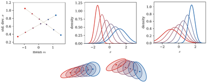
One- and two-dimensional Gaussian $\Wass_2$ geodesics. In one dimension, the coordinates $(m,\sigma)$ turn geodesics into Euclidean segments in the upper half-plane. In two dimensions, means move linearly while covariance ellipses follow the Bures--Wasserstein interpolation.

The two-dimensional Gaussian panels in the boxed figure show covariance ellipses evolving along the Bures--Wasserstein interpolation.

Interactive panel. Use the target mean, variance, and angle controls to see how the Gaussian Wasserstein geodesic moves means and covariance ellipses.

References¶

Monge, G. (1781). Mémoire sur la théorie des déblais et des remblais. Histoire de l’Académie Royale Des Sciences, 666–704.
Villani, C. (2003). Topics in Optimal Transportation (Vol. 58). American Mathematical Society.
Villani, C. (2009). Optimal Transport: Old and New (Vol. 338). Springer.
Santambrogio, F. (2015). Optimal Transport for Applied Mathematicians: Calculus of Variations, PDEs, and Modeling. Birkhäuser.
Rachev, S. T., & Rüschendorf, L. (1998). Mass Transportation Problems: Volume I: Theory. Springer.
Rudin, W. (1987). Real and Complex Analysis (Third). McGraw–Hill.
Bogachev, V. I. (2007). Measure Theory. Springer.
Reinhard, E., Adhikhmin, M., Gooch, B., & Shirley, P. (2001). Color Transfer between Images. IEEE Computer Graphics and Applications, 21(5), 34–41.
Pitié, F., Kokaram, A. C., & Dahyot, R. (2005). N-dimensional Probability Density Function Transfer and Its Application to Color Transfer. IEEE International Conference on Computer Vision, 1434–1439.
Rabin, J., Peyré, G., Delon, J., & Bernot, M. (2011). Wasserstein barycenter and its application to texture mixing. International Conference on Scale Space and Variational Methods in Computer Vision, 435–446.
Brenier, Y. (1987). Décomposition polaire et réarrangement monotone des champs de vecteurs. C. R. Acad. Sci. Paris Sér. I Math., 305(19), 805–808.
Brenier, Y. (1991). Polar factorization and monotone rearrangement of vector-valued functions. Communications on Pure and Applied Mathematics, 44(4), 375–417.
Gangbo, W., & McCann, R. J. (1996). The geometry of optimal transportation. Acta Mathematica, 177(2), 113–161.
McCann, R. J. (1997). A convexity principle for interacting gases. Advances in Mathematics, 128(1), 153–179.
Caffarelli, L. (2003). The Monge-Ampere equation and optimal transportation, an elementary review. Lecture Notes in Mathematics, Springer-Verlag, 1–10.