Divergences and Dual Norms

This chapter compares optimal transport with divergence-based and adversarial ways of measuring discrepancy. The main stake is topological: $\phi$-divergences are cheap but strong, while dual norms and GAN objectives can be weak enough to compare singular measures. The discussion connects classical information divergences Ciszár, 1967Ali & Silvey, 1966 with modern integral probability metrics and generative modeling Sriperumbudur et al., 2009Goodfellow et al., 2014Arjovsky et al., 2017.

from pathlib import Path
import sys

from IPython.display import Image as DisplayImage
from IPython.display import display

here = Path.cwd()
myst_dir = None
for candidate in [here, here.parent, here / "myst", here.parent / "myst", here.parent.parent / "myst"]:
    if (candidate / "ot4ml_web.py").exists():
        myst_dir = candidate.resolve()
        sys.path.insert(0, str(myst_dir))
        break

if myst_dir is None:
    raise RuntimeError("Could not locate myst/ot4ml_web.py")

repo_root = myst_dir.parent
thumbnails = repo_root / "notebooks-figures" / "thumbnails"

def show_book_figure(name, width=760):
    display(DisplayImage(filename=str(thumbnails / f"{name}.png"), width=width))

Dual Norms and Integral Probability Metrics¶

Dual norms generalize the $\Wass_1$ test-function principle. They are useful in statistics because they compare distributions by restricting the discriminator class.

Integral Probability Metrics¶

The Kantorovich--Rubinstein formula for $\Wass_1$ is a special case of a dual norm. This viewpoint designs weak discrepancies by testing signed differences of measures against a controlled class of functions.

The choice of the test-function class $B$ determines both the topology and the statistical behavior of the discrepancy Sriperumbudur et al., 2012Sriperumbudur et al., 2009Sriperumbudur et al., 2008.

show_book_figure("dualnorms-ipm-witnesses")

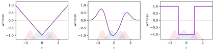
Dual witnesses for integral probability metrics. The red and blue curves are two one-dimensional probability densities and the violet curve is a normalized optimal dual witness $f^\star_{\alpha,\beta}$ for the IPM variational problem. $\Wass_1$ restricts the slope through Kantorovich--Rubinstein duality, MMD restricts the RKHS norm, and total variation can saturate pointwise and therefore reacts sharply to signed density differences.

The interactive demo makes the topology visible. As the two densities move, the total-variation witness jumps with the sign of the density difference, the Wasserstein witness keeps a unit-slope geometry, and the MMD witness is smoothed by the kernel bandwidth.

The following proposition gives a compact-space criterion. The dual ball should be rich enough to approximate continuous observables, but compact enough for weak convergence to imply uniform convergence over the discriminator class.

Dual RKHS Norms and Maximum Mean Discrepancies¶

Kernel methods turn probability measures into mean elements of a reproducing kernel Hilbert space. The resulting Hilbertian dual norms are quadratic discrepancies, handled with Euclidean geometry while retaining a weak test-function interpretation.

The conditional version is the right notion for probability distances, because one applies the quadratic form to signed measures $\xi=\alpha-\beta$ of total mass zero. Adding $a(x)+a(y)$ to the kernel does not change $\iint K(x,y)\,\d\xi(x)\,\d\xi(y)$ on such measures, and many natural distance kernels are only conditionally positive definite.

These norms are usually called maximum mean discrepancies in statistics and machine learning Gretton et al., 2012Muandet et al., 2017, and kernel norms in shape analysis Hofmann et al., 2008. If $X,X'$ are independent with law $\alpha$, then $\norm{\alpha}_K^2=\EE_{X,X'}(K(X,X'))$, whenever this expression is finite.

Further background on RKHS spaces can be found in Berlinet & Thomas-Agnan, 2003Hofmann et al., 2008Schölkopf & Smola, 2002.

In the special case where $\alpha=\sum_{i=1}^n a_i\delta_{x_i}$ is discrete, one obtains

where $(K_X)_{i,i'}=K(x_i,x_{i'})$. In particular, if $\alpha=\sum_i a_i\delta_{x_i}$ and $\beta=\sum_i b_i\delta_{x_i}$ are supported on the same point cloud, then $\norm{\alpha-\beta}_K^2=(a-b)^\top K_X(a-b)$, a Euclidean quadratic form on the simplex. For two arbitrary discrete measures,

Phi-Divergences¶

This section develops divergences based on pointwise density ratios. They are computationally simple and statistically classical, but they do not see small spatial displacements between singular measures.

Definition by Density Ratios¶

Phi-divergences are simpler to compute, typically $O(n)$ for discrete distributions, but they never metrize weak-$\ast$ convergence on singular measures. Another route is possible through Bregman divergences, which may metrize weak-$\ast$ convergence when the associated entropy functional is weakly regular.

If $\phi'_\infty=+\infty$, then $\phi$ grows faster than any linear function and is called superlinear. Any entropy function induces a $\phi$-divergence, also known as a Ciszar divergence or $f$-divergence Ciszár, 1967Ali & Silvey, 1966.

Here $\alpha^\perp$ is the part of $\alpha$ singular with respect to $\beta$. The singular term is the recession contribution of the perspective functional. It gives the weak-$\ast$ lower-semicontinuous extension of the density-ratio integral when singular mass appears. This is essential for linear-growth entropies such as total variation. For superlinear entropies, such as the usual entropy, $\phi'_\infty=+\infty$, so the divergence is infinite when $\alpha$ is not absolutely continuous with respect to $\beta$.

For discrete measures supported on the same set,

the formula becomes

Classical Examples and Topology¶

The following examples calibrate the strength of $\phi$-divergences. KL is sensitive to absolute continuity, while total variation gives the strong topology and therefore behaves very differently from Wasserstein-type weak metrics.

Main Families of $\phi$-Divergences¶

Several classical divergences fit in the same template. The power-divergence family

interpolates between the Pearson $\chi^2$ divergence at $\gamma=2$, a Hellinger-type behavior at $\gamma=1/2$, and, by taking limits, the KL divergence as $\gamma\to1$ and the reverse KL or Burg entropy $\phi_0(s)=-\log s+s-1$ as $\gamma\to0$. The Hellinger divergence is often written with $\phi_H(s)=(\sqrt{s}-1)^2$; for measures with densities, $\operatorname{Hellinger}(\alpha,\beta) =\norm{\sqrt{\rho_\alpha}-\sqrt{\rho_\beta}}_{L^2}$. The Jensen--Shannon divergence is the symmetrized and bounded KL-to-the-mixture divergence

generated, up to an irrelevant affine term, by $\phi_{\operatorname{JS}}(s)=s\log s-(s+1)\log((s+1)/2)$. Total variation, generated by $|s-1|$, is exceptional because it is both a $\phi$-divergence and an integral probability metric.

show_book_figure("dualnorms-phi-generators")

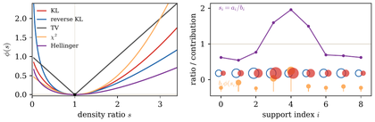
$\phi$-divergences through density ratios. The left panel shows normalized generators for common divergences as functions of $s=\d\alpha/\d\beta$; all curves vanish at $s=1$ up to affine normalization. The right panel shows the discrete formula $D_\phi(a|b)=\sum_i b_i\phi(a_i/b_i)$: hollow blue circles encode $b_i$, filled red circles encode $a_i$, the violet curve gives the ratios $a_i/b_i$, and orange lollipops show local KL-type contributions.

The interactive demo changes the generator family and the amount of mismatch between two discrete histograms. The near-zero control deliberately creates small target bins, making the recession and singularity behavior visible: ratio-based penalties react to overlap and density ratios rather than to spatial displacement.

Variational Dual Formula¶

The following formula turns a pointwise density-ratio penalty into a dual optimization problem over test functions. It is the analogue, for $\phi$-divergences, of the Kantorovich dual formula for transport costs.

GANs via Duality¶

GANs fit naturally into the dual viewpoint: the discriminator is a parameterized potential and the generator moves a reference measure. This section first explains the original divergence-based GAN objective, then contrasts it with integral probability metrics such as MMD and Wasserstein distances.

The goal is to fit a generative parametric model $\alpha_\theta=(g_\theta)_\sharp\zeta$ to empirical data

where $\zeta$ is a fixed density over the latent space and $g_\theta:\mathcal{Z}\to\X$ is the generator, often a neural network.

Divergence-Based Adversarial Losses¶

Any $\phi$-divergence can be written in adversarial form through the dual formula:

Replacing the unrestricted potential $f$ by a neural network $f_\xi$ gives a saddle problem

The original vanilla GAN Goodfellow et al., 2014 is this construction for the Jensen--Shannon generator

up to affine normalizations and the usual reparametrization of the potential by a discriminator with values in $(0,1)$. In practice the min--max problem is solved by alternating stochastic gradient descent/ascent. Unlike the convex-concave variational formula, the neural parametrization is nonconvex in $\theta$ and nonconcave in $\xi$, which explains instability and mode-collapse pathologies. These losses estimate density ratios, which is meaningful when the measures overlap but can saturate when the model and data are mutually singular. For example, the Jensen--Shannon divergence is already maximal for disjoint supports.

Dual Norms and Integral Probability Metrics¶

Instead of a density-ratio divergence, one can minimize an integral probability metric:

MMD-GANs take $B$ to be a unit ball in an RKHS Dziugaite et al., 2015; Wasserstein GANs take $B$ to be a Lipschitz ball, following Kantorovich--Rubinstein duality Arjovsky et al., 2017Frogner et al., 2015. The advantage is topological: for bounded continuous RKHS balls, or for bounded Lipschitz balls on compact spaces, the objective is weakly continuous. It can therefore compare singular empirical and generated measures through test functions instead of requiring pointwise density ratios. The price is that the discriminator class must be controlled geometrically, either by a kernel norm, a Lipschitz constraint, or a related regularization.

Wasserstein GANs originally used weight clipping as a proxy for enforcing $f_\xi\in\{f:\operatorname{Lip}(f)\le1\}$. This parameter set is both smaller than the true Lipschitz ball and nonconvex, so clipping should be understood as a practical heuristic rather than a faithful implementation of the Kantorovich--Rubinstein dual constraint.