Dual Problem

Duality turns the transport problem into a search for potentials rather than couplings. This chapter explains why potentials certify optimality, how $c$-transforms regularize them, and why the quadratic case reveals convex analysis behind Brenier maps. Linear-programming duality gives the discrete picture Bertsimas & Tsitsiklis, 1997, while the continuous form is one of the central theorems of optimal transport Villani, 2003Santambrogio, 2015.

from pathlib import Path
import sys

from IPython.display import Image as DisplayImage
from IPython.display import display

here = Path.cwd()
myst_dir = None
for candidate in [here, here.parent, here / "myst", here.parent / "myst", here.parent.parent / "myst"]:
    if (candidate / "ot4ml_web.py").exists():
        myst_dir = candidate.resolve()
        sys.path.insert(0, str(myst_dir))
        break

if myst_dir is None:
    raise RuntimeError("Could not locate myst/ot4ml_web.py")

repo_root = myst_dir.parent
thumbnails = repo_root / "notebooks-figures" / "thumbnails"

def show_book_figure(name, width=760):
    display(DisplayImage(filename=str(thumbnails / f"{name}.png"), width=width))

Discrete Dual¶

The discrete dual gives finite-dimensional certificates of optimality. Its complementary-slackness conditions identify where an optimal coupling can put mass.

The two vectors play the role of source and target prices; admissibility means that no transported pair is priced above its travel cost. The discrete Kantorovich problem is a linear program. Hence its value can be computed either by minimizing over couplings or by maximizing over a pair of dual vectors.

The primal-dual optimality relation locates the support of an optimal plan. If $P$ is optimal and $(f,g)$ is optimal, then

Thus potentials are not transport maps themselves. They are certificates, and their equality set with the cost matrix is where an optimal coupling is allowed to place mass.

show_book_figure("dual-kantorovich-discrete-potentials")

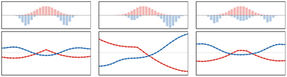
Discrete Kantorovich dual potentials for the quadratic cost $C_{ij}=|x_i-y_j|^2$. The upper strip shows the fixed source histogram in red and the target histogram in blue. The lower strip shows optimal dual vectors $(f,g)$, with a gauge chosen so that $\langle f,a\rangle=0$. Complementary slackness states that mass can be transported only through entries where $f_i+g_j=C_{ij}$.

The interactive demo varies the target law and the number of bins. The lower curves are reconstructed from the active monotone transport graph, so the equality set moves as the coupling support changes.

The formula (2) also shows that $(a,b)\mapsto\mathcal{L}_C(a,b)$ is convex, being a supremum of linear functions. From the primal formulation, $C\mapsto\mathcal{L}_C(a,b)$ is concave.

Auction Algorithm and Dual Prices¶

Assignment algorithms become more transparent once one has dual variables. The auction algorithm is a dual-price method: it updates target prices and maintains an approximate complementary-slackness certificate. The tolerance $\varepsilon$ removes ties, stabilizes price updates, and gives a quantitative optimality certificate Bertsekas, 1981Bertsekas, 1992Mérigot & Thibert, 2020.

Consider the square assignment problem with costs $C_{ij}$ and rewrite it as a profit maximization problem with $a_{ij}=-C_{ij}$. The auction algorithm keeps prices $p_j$ on the target points and a partial assignment. For an unassigned source $i$, define the best and second-best reduced profits

Source $i$ bids for $j_i$ and increases its price by the gap to the second-best target, plus a margin:

The target $j_i$ is assigned to $i$, and its previous owner, if any, becomes unassigned. The iteration stops when all sources are assigned.

show_book_figure("dual-auction-progression")

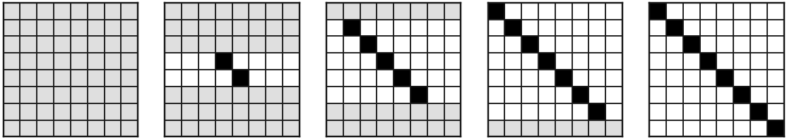
Matrix view of actual auction iterates on a diagonally dominant one-dimensional squared-distance assignment. Each panel records the current ownership state: unassigned bidders are shown as flat rows, while assigned bidders are shown as one-hot rows at their currently held target. The snapshots show initialization, intermediate price updates, and the final identity assignment satisfying complementary slackness.

The interactive auction view exposes the price dynamics directly. Increasing $\varepsilon$ makes bids coarser and the final certificate looser; decreasing it makes the price landscape closer to exact complementary slackness.

For fixed prices $p$, eliminating the bidder utilities $u_i$ in the dual minimization gives the convex objective

which comes from the dual constraints $u_i+p_j\ge a_{ij}$. The auction update should therefore be viewed as a price-adjustment method on this nonsmooth dual landscape, rather than as a generic gradient step.

During the bidding process, the last bid made by a source makes its chosen target better, up to the margin $\varepsilon$, than all alternatives. Subsequent price increases can only make targets less attractive, and one checks by induction that currently assigned pairs satisfy $\varepsilon$-complementary slackness. A standard finite-termination proof normalizes prices by subtracting their minimum, observes that each bid increases one target price by at least $\varepsilon$, and bounds the normalized price spread in terms of the range of the profits.

General Formulation¶

The continuous dual is the analytic counterpart of the discrete linear program. It uses continuous potentials because measures are naturally probed through integration. The pairing is $\langle f,\alpha\rangle\eqdef\int f\,\d\alpha$.

The discrete case corresponds to dual vectors that are samples of continuous potentials, $(f_i,g_j)=(f(x_i),g(y_j))$. The primal-dual support condition becomes

For the one-dimensional quadratic cost, the continuous potentials can be read from the monotone map $T=F_\beta^{-1}\circ F_\alpha$: on the active graph, $f'(x)=2(x-T(x))$ and $g=f^c$.

show_book_figure("dual-kantorovich-continuous-potentials")

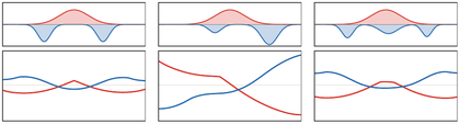
Continuous Kantorovich potentials for the same source and target families as the discrete potential figure. The upper strips show the source density $\alpha$ in red and the target density $\beta$ in blue. The lower strips show potentials $f$ and $g=f^c$ for the quadratic cost $c(x,y)=|x-y|^2$. The equality set $f(x)+g(y)=c(x,y)$ contains the monotone transport graph.

The interactive view computes the monotone map from numerical quantiles and then integrates $f'(x)=2(x-T(x))$. It makes clear that the potentials change smoothly with the target law, even though the equality set remains a thin transport graph.

In contrast to the primal problem, showing existence of solutions to the continuous dual is nontrivial: the constraint set is not compact and the objective is not coercive. The machinery of $c$-transforms repairs this by replacing arbitrary potentials with regular best responses.

c-Transforms¶

The $c$-transform is the operation that improves potentials without changing feasibility. It is both a proof device for dual attainment and the route from duality to Brenier’s convex potentials.

Best-Response Potentials¶

Keeping a dual potential $f$ fixed, one can maximize in closed form over the second potential in the dual problem:

The constraint is equivalent to $g(y)\le f^c(y)$.

Since $\beta$ is positive, maximizing $\int g\,\d\beta$ is achieved by taking $g=f^c$ on the support of $\beta$, equivalently $\beta$-almost everywhere.

show_book_figure("dual-c-transform-envelope")

Discrete $c$-transform as a lower envelope for costs $c_p(x,y)=|x-y|^p$. The red circles are four source atoms $x_i$ with potential values $f_i$; the gray curves are $y\mapsto c_p(x_i,y)-f_i$; the colored curve is their lower envelope $f^c(y)=\min_i c_p(x_i,y)-f_i$. This is the semi-discrete situation where the source space is finite.

The interactive envelope view exposes the exponent, the number of atoms, and the potential amplitude. This is the local mechanism behind many dual regularity statements: taking a pointwise minimum of translated costs inherits regularity from the cost.

The map $(f,g)\mapsto(g^{\bar c},f^c)$ replaces dual potentials by better ones: it preserves feasibility and improves the dual objective. Functions of the form $f^c$ and $g^{\bar c}$ are called $c$-concave and $\bar c$-concave functions. These partial minimizations define maximizers on the supports of $\alpha$ and $\beta$, while the transform itself defines functions on the whole ambient spaces. This gives a canonical extension of dual solutions beyond their active supports.

This stability is crucial for dual attainment. When $c$ is Lipschitz on compact spaces, one can replace arbitrary admissible potentials by $c$-transformed ones with a uniform Lipschitz bound; after fixing the harmless additive gauge, compactness follows from Arzela--Ascoli.

Euclidean Case¶

The Euclidean quadratic cost is the model case where $c$-transforms become ordinary convex conjugates after removing quadratic terms. This is the algebraic bridge between Kantorovich duality and Brenier maps.

The cost $c(x,y)=-\langle x,y\rangle$ on $\X=\Y=\RR^d$ is central because it reduces the quadratic Wasserstein problem to convex duality. Indeed, for any $\pi\in\Couplings(\alpha,\beta)$,

For $c(x,y)=-\langle x,y\rangle$,

Thus $c$-concave functions are negatives of convex functions. In the one-dimensional bilinear model case, the hard double $c$-transform is an operation of taking concave envelopes.

Failure of Alternating Optimization¶

A crucial property of the Legendre transform is that $f^{***}=f^*$, and that $f^{**}$ is the convex envelope of $f$. These properties carry over to $c$-transforms Rockafellar, 2015.

This invariance property shows that one can improve only once by exact alternating maximization:

Thus the method reaches a stationary point immediately. This is the classical failure mode of alternating maximization on a nonsmooth problem, where the nonsmooth constraint mixes the two variables. The workaround is to introduce smoothing, which the next chapters develop through entropic regularization and Sinkhorn scaling.

For the bilinear cost $c(x,y)=-xy$ on a compact interval, $c$-concave functions are ordinary concave functions and $f^{c\bar c}$ is the smallest concave majorant of $f$. A hard transform removes non-concave oscillations in one closure step instead of producing a gradual ascent.

show_book_figure("dual-alternating-c-transform-failure")

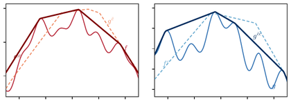
Hard $c$-transforms for the bilinear cost $c(x,y)=-xy$. Dark curves are the double-transform closures $f^{c\bar c}$ and $g^{\bar c c}$, which are concave majorants, while dashed lighter curves are the one-sided best responses $g^{\bar c}$ and $f^c$ after a harmless vertical gauge shift. Exact alternating best responses are useful for certificates but do not give the smooth iterative dynamics later provided by entropic regularization.

The final interactive demo turns this algebra into a visible operation: change the roughness of the starting potential and observe that the hard double transform jumps directly to its concave closure.