Optimal Matching between Point Clouds

This opening chapter isolates the simplest form of optimal transport: pairing two finite point clouds. The stakes are algorithmic and geometric at once: one sees the combinatorial nature of transport, the special simplicity of the line, and the first hints that convex relaxation will be necessary in higher dimension. Classical assignment algorithms such as the Hungarian method and auction methods Kuhn, 1955Bertsekas, 1992 provide the computational backdrop, while the geometric examples prepare the Kantorovich relaxation.

from pathlib import Path
import sys

from IPython.display import Image as DisplayImage
from IPython.display import display

here = Path.cwd()
myst_dir = None
for candidate in [here, here.parent, here / "myst", here.parent / "myst", here.parent.parent / "myst"]:
    if (candidate / "ot4ml_web.py").exists():
        myst_dir = candidate.resolve()
        sys.path.insert(0, str(myst_dir))
        break

if myst_dir is None:
    raise RuntimeError("Could not locate myst/ot4ml_web.py")

repo_root = myst_dir.parent
thumbnails = repo_root / "notebooks-figures" / "thumbnails"

def show_book_figure(name, width=760):
    display(DisplayImage(filename=str(thumbnails / f"{name}.png"), width=width))

# Static figures are Python-rendered; interactive demos are browser-rendered.
from ot4ml_web import (
    plot_histogram_equalization,
    plot_cost_power_sweep,
    plot_quantile_matching,
    plot_regularization_sweep,
)

Monge Problem for Discrete Points¶

This section formulates matching as Monge’s deterministic transport problem on two equally weighted clouds. The one-dimensional case is a transparent reference case where the optimal map can be read off by sorting.

Matching Problem¶

Given a cost matrix $(C_{i,j})_{i \in \{1,\ldots,n\}, j \in \{1,\ldots,m\}}$ and assuming $n=m$, the optimal assignment problem aims to find a bijection $\sigma$ within the set $\Perm(n)$ of permutations of $n$ elements that solves

One could naively evaluate the cost above for all permutations in $\Perm(n)$. However, this set has size $n!$, which becomes enormous even for small values of $n$. In general, the optimal $\sigma$ is not unique.

One-Dimensional Case¶

In one dimension, convex costs select monotone matchings.

This property extends by continuity to convex costs that are not strictly convex, such as $|x-y|$, but then the matching is not necessarily unique. For convex costs, the algorithm to compute an optimal transport is to sort the points: find permutations $\sigma_X,\sigma_Y$ such that

and then map $x_{\sigma_X(k)}$ to $y_{\sigma_Y(k)}$. Equivalently, an optimal transport is $\sigma=\sigma_Y\circ\sigma_X^{-1}$. The computational cost is therefore $O(n\log n)$, using for instance quicksort.

If the distance profile is concave instead of convex, the geometry changes. For costs such as $c_p(x,y)=|x-y|^p$ with $0<p<1$, splitting a displacement into several smaller displacements is expensive, so optimal matchings tend to create long exchanges rather than the monotone equal-rank pairing. This is the strictly concave regime studied by Gangbo and McCann Gangbo & McCann, 1996.

The real line still gives special structure. After sorting all red and blue points together, the ordered sequence decomposes into maximal alternating chains, and local matching indicators can certify pairs that must be matched in an optimum. Removing such certified pairs and repeating yields an exact hierarchical algorithm for the unit-mass balanced assignment problem, with worst-case complexity $O(n^2)$ in the framework of Delon, Salomon and Sobolevski Delon et al., 2012. Very concave costs also motivate simpler greedy heuristics, studied for instance by Ottolini and Steinerberger Ottolini & Steinerberger, 2023. The point is that these methods are not generic linear-programming solvers; they use the one-dimensional order and the concavity of the distance profile.

show_book_figure("matching-1d-convex-concave-costs")

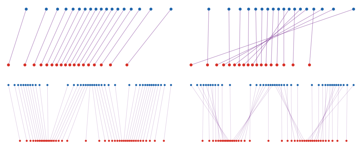
One-dimensional assignments for ordered source and target clouds with costs $c_p(x,y)=|x-y|^p$. The top row uses single-Gaussian source and target clouds; the bottom row uses a denser two-component source and three-component target. For the convex quadratic cost, equal ranks are matched and the segments do not cross. For the concave cost, the optimum creates long crossing exchanges; the ordered line remains useful, but through the alternating-chain structure of concave transport rather than through monotone rearrangement.

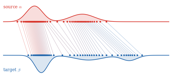
The next figure shows the monotone case more explicitly. The red and blue curves are smooth laws used to generate equal-weight empirical measures; the dots are inverse-CDF samples at common quantile levels. The monotone assignment connects equal ranks.

show_book_figure("matching-1d-quantile-assignment")

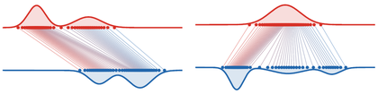
One-dimensional optimal matching by quantile sorting. The red and blue curves are smooth laws used to generate equal-weight empirical measures; the dots are inverse-CDF samples at common quantile levels. The monotone assignment connects equal ranks, both for two Gaussian mixtures and for the transport from one central Gaussian toward a three-mode target law.

The interactive panel exposes the point count and the two laws while keeping the monotone equal-rank construction in the background.

n_points = 52
source_law = "two"      # one, two, wide_two, three
target_law = "three"    # one, two, wide_two, three

fig = plot_quantile_matching(
    n=n_points,
    source=source_law,
    target=target_law,
)

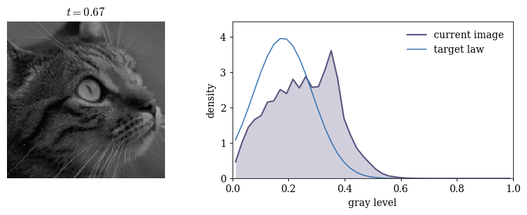
If $\phi:\RR\to\RR$ is increasing, the same technique applies to costs of the form $h(|\phi(x)-\phi(y)|)$ after a change of variable. A typical application is grayscale histogram equalization. The empirical cumulative distribution of image luminance values is transported to a prescribed target histogram, for instance a concentrated or reference-image histogram. In one dimension, the monotone rearrangement gives the exact transport map, so the operation is both computationally simple and geometrically faithful: it matches distributions of intensities rather than individual pixels.

show_book_figure("monge-histogram-equalization")

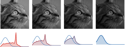
Histogram equalization as one-dimensional Monge transport on pixel intensities. The map is the monotone rearrangement $T=Q_\beta\circ F_\alpha$; here $\beta$ is a truncated Gaussian concentrated near dark intensities. The images are interpolated pointwise by $I_t=(1-t)I+tT(I)$, and all histograms share the same vertical scale.

The interactive view below exposes the target mean, target standard deviation, and interpolation time.

target_mean = 0.18
target_sigma = 0.105
interpolation = 0.67  # 0 is the original image, 1 is fully equalized

fig = plot_histogram_equalization(
    target_mean=target_mean,
    target_sigma=target_sigma,
    interpolation=interpolation,
)

If $h$ is strictly convex, then all optimal assignments are increasing, and if the points are all distinct, this increasing map is unique. If $h$ is not strictly convex, for instance $c(x,y)=|x-y|$, non-increasing optimal assignments can also exist. This happens, for example, in the book-shifting problem with overlapping uniform distributions, where the mass in the intersection can stay fixed.

Optimal Transport on the Circle¶

The sorting rule on the line has a periodic analogue. Identify the circle with $\mathbb S^1=\RR/\mathbb Z$, let

The only extra datum, compared with the line, is where one opens the circle. Once a cut has been chosen, the circle is unfolded into an interval and the one-dimensional monotone assignment can be used. In the discrete case, changing the cut is the same as applying a cyclic shift to one of the two circular orderings.

show_book_figure("monge-circle-cut-unfolding")

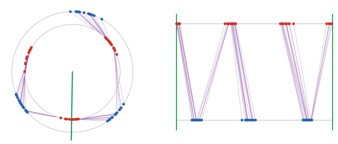
Optimal transport on the circle by cutting and unfolding. Purple segments show the optimal matching and the green radius marks the chosen cut. The red and blue atoms live on two copies of the circle; the denser point clouds make the cyclic ordering visible. Once the circle is opened at this angle, the same matching appears as a monotone one-dimensional assignment on the interval, with the two green endpoints identified.

show_book_figure("matching-2d-cost-exponent")

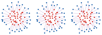
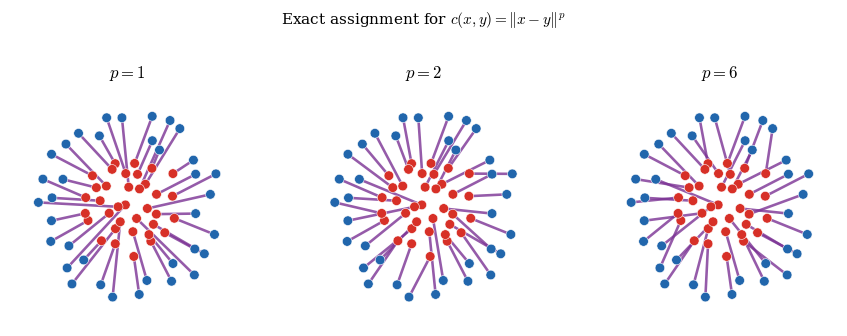
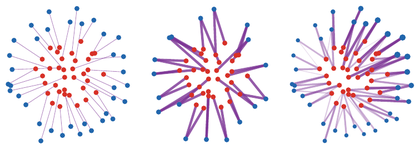
Optimal assignments between the same two point clouds for three powers of the Euclidean distance. The source atoms are semi-regular samples in a central disk, while the target atoms are semi-regular samples on a thin annulus; this canonical geometry is reused in later coupling and regularization figures. The feasible set is unchanged, but increasing $p$ penalizes the longest edges more strongly and changes the global organization of the permutation.

The interactive panel reuses the same disk-to-annulus geometry and exposes the number of points, the data geometry, and the cost exponents $p$ in $c(x,y)=\norm{x-y}^p$.

n_points_2d = 36
source_shape = "disk"       # disk, annulus, two_blobs, three_blobs, crescent
target_shape = "annulus"    # disk, annulus, two_blobs, three_blobs, crescent
cost_powers = (1, 2, 6)
seed = 2074

fig = plot_cost_power_sweep(
    n_points=n_points_2d,
    source_shape=source_shape,
    target_shape=target_shape,
    cost_powers=cost_powers,
    seed=seed,
)

Rational Weights¶

The strict assignment model is also tied to equal cardinalities and equal weights. As soon as the target resolution changes or the weights are not uniform, a permutation no longer describes the feasible transports. One instead needs a nonnegative transport matrix with prescribed row and column sums; this is the finite-dimensional Kantorovich relaxation developed in the next chapters.

show_book_figure("matching-resolution-and-weights")

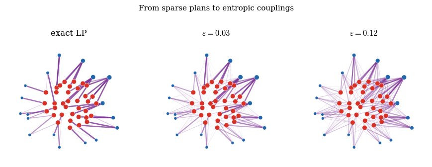
From assignments to transport plans, using the same disk-to-annulus geometry. In the balanced equal-weight case, each source atom is matched to one target atom. With a target cloud that has half as many atoms, or with strongly nonuniform target weights, the coupling matrix can merge or split mass; segment thickness and opacity encode its nonzero entries, and blue marker areas encode the prescribed target masses.

The interactive panel below exposes the target resolution, target weights, and regularization level. The first displayed plan is sparse, while positive regularization values show the entropic smoothing used later in the Sinkhorn chapter.

n_source = 36
n_target = 18
weight_mode = "angular"     # uniform, angular, right_heavy
weight_strength = 1.4
epsilons = (0.0, 0.03, 0.12)

fig = plot_regularization_sweep(
    n_source=n_source,
    n_target=n_target,
    source_shape="disk",
    target_shape="annulus",
    cost_power=2,
    epsilons=epsilons,
    weight_mode=weight_mode,
    weight_strength=weight_strength,
    seed=2031,
)

show_book_figure("matching-rational-duplication")

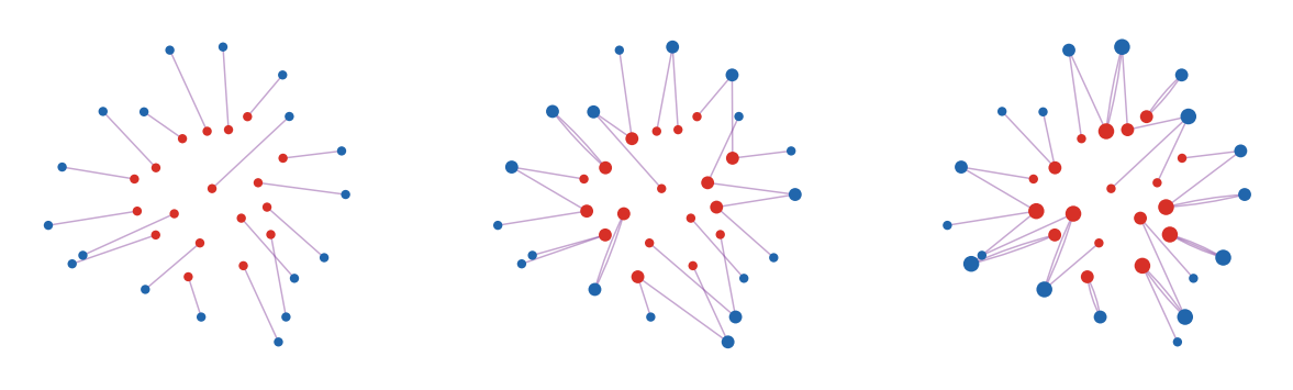
Rational weights as duplicated uniform matchings, using the same disk-to-annulus geometry with fewer displayed atoms. The red and blue locations are kept fixed, while disk areas encode the integer multiplicities $k_i$ and $\ell_j$. Solving the assignment problem after duplicating particles produces several collapsed segments attached to high-multiplicity atoms; this is the integer count matrix of the proposition.

Two-Dimensional Assignments¶

This efficient strategy to compute the OT in one dimension does not extend to higher dimensions. In two dimensions, as already noted by Monge, optimal segments for the Euclidean distance cannot cross.

This property alone is not enough to lead to an efficient algorithm. Non-crossing is only a necessary local test, not a compact certificate of optimality. For instance, if $n$ sources and $n$ targets are placed alternately on the boundary of a convex polygon, the number of non-crossing perfect matchings is the Catalan number

Thus even after forbidding crossings, an exhaustive search remains exponential. The two-segment swap in the proof above is nevertheless useful: it explains why a crossing matching cannot be optimal, but it does not select among the exponentially many planar matchings that survive this local test.

Matching Algorithms¶

This section briefly locates matching within classical combinatorial optimization. Its main point is that efficient algorithms exist, but their cleanest analysis is obtained only after introducing the linear-programming viewpoint.

Efficient algorithms exist to solve the optimal matching problem. The most well-known are the Hungarian method and auction algorithms Kuhn, 1955Bertsekas, 1981Bertsekas, 1992. Auction algorithms use prices on the target points: each source bids for the target with largest reduced profit, the target price is increased, and the process terminates when the $\epsilon$-complementary slackness conditions are satisfied. For integer costs, choosing $\epsilon<1/n$ gives an exact optimum after a finite number of bids Bertsekas, 1992. The dual chapter revisits this algorithm after Kantorovich duality and explains why it is a dual price method, parallel in spirit to Sinkhorn scaling.

Hungarian Primal-Dual Method¶

The Hungarian method is best understood as a certificate-building algorithm for the assignment linear program. It maintains a partial matching $M$ and dual prices $(u_i,v_j)$ satisfying

The equality graph $E(u,v)=\{(i,j):u_i+v_j=C_{i,j}\}$ contains the edges whose reduced cost is zero. The algorithm only augments $M$ along alternating paths made of equality edges. Starting from an unmatched source, it grows an alternating tree with source set $S$ and target set $T$. If the tree reaches an unmatched target, the matching is augmented along the path. If no such edge exists, the dual variables are shifted by the smallest slack

This update preserves all inequalities $u_i+v_j\leq C_{i,j}$, keeps the current alternating tree tight, and creates at least one new equality edge leaving $S$. Maintaining these slacks incrementally gives the standard $O(n^3)$ implementation for an $n\times n$ assignment problem.

The following figure summarizes actual iterates by displaying only the evolving partial assignment: unmatched rows are shown as flat rows to keep a fixed matrix format, and matched rows are shown as one-hot rows.

show_book_figure("matching-hungarian-progression")

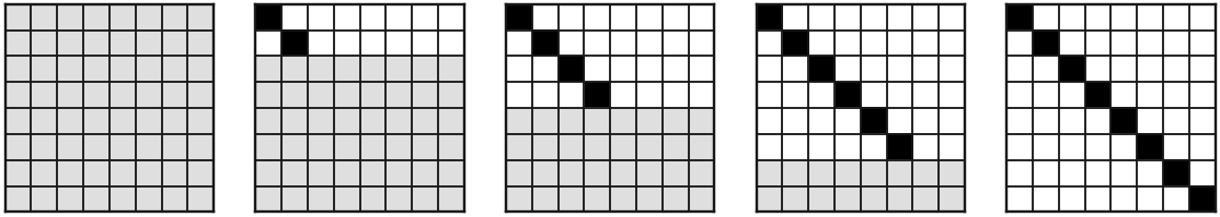
Matrix view of actual Hungarian primal-dual iterates on a diagonally dominant ordered one-dimensional squared-distance assignment. Each panel records the current partial assignment state: unassigned rows are kept flat, while assigned rows are one-hot. The snapshots are taken at initialization and after two, four, six and eight augmentations; for this pedagogical instance the partial assignments grow along the diagonal, and the final matrix is the identity assignment certified by complementary slackness.