Wasserstein Gradient Flows

Once $\Wass_2$ is a dynamic metric, one can run gradient descent directly on the space of measures. This chapter derives the formal Wasserstein gradient, explains the JKO minimizing-movement scheme, records the role of geodesic convexity in convergence, and then applies the same calculus to mean-field neural-network training.

from pathlib import Path
import sys

from IPython.display import Image as DisplayImage
from IPython.display import display

here = Path.cwd()
myst_dir = None
for candidate in [here, here.parent, here / "myst", here.parent / "myst", here.parent.parent / "myst"]:
    if (candidate / "ot4ml_web.py").exists():
        myst_dir = candidate.resolve()
        sys.path.insert(0, str(myst_dir))
        break

if myst_dir is None:
    raise RuntimeError("Could not locate myst/ot4ml_web.py")

repo_root = myst_dir.parent
thumbnails = repo_root / "notebooks-figures" / "thumbnails"

def show_book_figure(name, width=760):
    display(DisplayImage(filename=str(thumbnails / f"{name}.png"), width=width))

Minimizing Movements and Wasserstein Gradients¶

This first section explains how a variational implicit-Euler step on measures gives rise, in the small-step limit, to a continuity equation driven by the Wasserstein gradient of the energy.

We consider a function $f(\alpha)$ and seek a minimizing evolution $(\alpha_t)_t$. The minimizing-movement strategy over a metric space builds a discrete-time evolution using an implicit Euler scheme:

Euclidean Gradient Flows¶

If (1) is restricted to finite dimensions with $\alpha_t=\delta_{x(t)}$ and $\alpha=\delta_x$, it becomes the implicit Euler scheme

Its solution is formally

In contrast, explicit Euler uses

Both schemes converge as $\tau\to0$ to the classical gradient flow

Wasserstein Gradient Formula¶

The implicit Euler scheme has the advantage that it does not require $h$ or $f$ to be smooth. For $f$, this is crucial when evolutions over measures may have densities, atoms or other singular parts.

As $\tau\to0$, under suitable conditions on $f$, (1) defines a continuous evolution $t\mapsto\alpha_t$. As in the dynamic formulation, this evolution can be described by a Lagrangian evolution. We use the following first-variation convention: for any $\beta\in\Pp(\RR^d)$ and the signed zero-mass perturbation $\rho=\beta-\alpha$,

The key infinitesimal object is the vector field that represents this differential in the Wasserstein metric.

The associated formal gradient flow is the continuity equation

The following proposition explains why this vector field is the Riemannian gradient for the $L^2(\alpha)$ metric on velocities.

The Wasserstein gradient-flow viewpoint already appears in John D. Lafferty’s PhD work, published as “The Density Manifold and Configuration Space Quantization”, under the name “density manifold”. It was then systematically developed by Otto, who exposed the formal Riemannian structure of this space Otto, 2001. Rigorous metric-space treatments and numerical JKO schemes can be found in Ambrosio et al., 2006Benamou et al., 2016Peyré, 2015Gallouët & Monsaingeon, 2017.

From the JKO Step to the Velocity Field¶

A first-order expansion of the JKO step explains why (8) uses the vector field $\Wgrad f(\alpha)$. Write (1) as a minimization over displacement fields $v$ such that $\alpha=(\Id+\tau v)_\sharp\alpha_t$:

The push-forward and energy expansions are

and hence

Thus the problem minimized in (1) has the first-order expansion

The pointwise minimizer is $v=-\Wgrad f(\alpha_t)$, which gives the velocity in the continuity equation. We now detail examples of such Wasserstein gradient flows.

show_book_figure("gradflow-jko-entropy-steps")

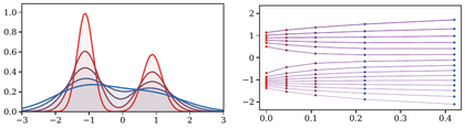
JKO minimizing movements for the entropy flow in one dimension. The left panel displays successive implicit-Euler minimizers for the heat equation, colored from red to blue. The right panel tracks inverse CDF values $Q_t(s)=F_t^{-1}(s)$ for selected probability levels $s$, giving a Lagrangian view of the proximal movement in Wasserstein space.

The interactive demo uses the heat-flow representative of the entropy JKO scheme: changing the step size changes the spacing between implicit Euler iterates, while the quantile panel shows how the same movement is seen in Lagrangian coordinates.

Discrete Evolutions¶

If $f(\alpha)$ can be evaluated on discrete distributions and $\Wgrad$ is continuous in this case, the flow (8) maintains the number of Dirac masses:

The particles $X(t)=(x_i(t))_i$ evolve according to the coupled ODE

where $F(X)=f\left(\frac1n\sum_i\delta_{x_i}\right)$. The factor $n$ comes from the empirical Wasserstein metric $\frac1n\sum_i\norm{\dot x_i}^2$.

Linear Functionals¶

The simplest example is a linear functional

Here $\delta f(\alpha)=h$ is independent of $\alpha$. The flow (8) becomes

Thus particles move independently according to the usual gradient flow (5).

Shannon Neg-Entropy¶

A very different behavior is obtained by considering functionals that require $\alpha_t$ to have a density. The canonical example is Shannon neg-entropy

Here $\delta f(\alpha)=\log(\frac{\d\alpha}{\d x})$ up to an additive constant, so $\Wgrad f(\alpha)=\nabla\alpha/\alpha$, often called the score. The flow (8) becomes the heat equation

Other entropy functionals lead to nonlinear diffusion equations; finite-volume and particle discretizations are discussed in Carrillo et al., 2015Gianazza et al., 2009Maas, 2011Erbar, 2010.

For example, a generalized entropy

for a scalar convex function $g$ leads, in the smooth-density regime, to

where the pressure $P$ satisfies $P'(s)=s g''(s)$. For $g(s)=s\log s$, one has $P(s)=s$ and recovers (23); for $g(s)=s^m/(m-1)$ with $m>1$, one obtains $P(s)=s^m$ up to an additive constant and the porous-medium equation.

A celebrated theorem by McCann McCann, 1997 states that an internal energy of the form (25), for $g:\RR^+\to\RR\cup\{+\infty\}$ with $g(0)=0$, is geodesically convex on $\Pp(\RR^d)$ when $g$ is convex and the map $r\mapsto r^d g(r^{-d})$ is convex and nonincreasing on $(0,+\infty)$. Examples include $g(s)=s^q$ for $q>1$ and Shannon entropy $g(s)=s\log s$. By contrast, $g(s)=-\log s$, associated with the reverse KL divergence, does not satisfy this displacement-convexity criterion.

show_book_figure("gradflow-heat-versus-porous-medium")

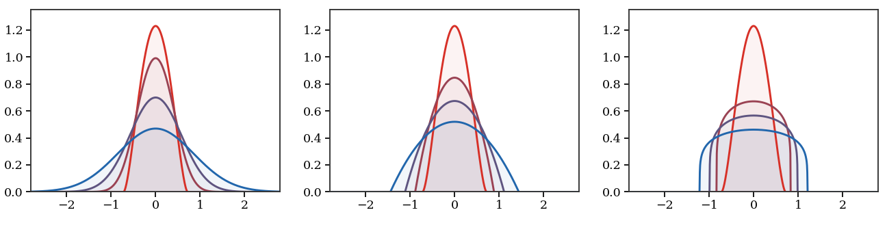
Entropy-driven Wasserstein gradient flows from the same compact initial density. The heat flow is generated by Shannon entropy $g(\rho)=\rho\log\rho$ and instantly develops Gaussian tails. The porous-medium flows use the power entropy $g(\rho)=\rho^m/(m-1)$, hence $\partial_t\rho=\Delta(\rho^m)$: the middle panel has $m=2$, while the right panel has the stronger nonlinearity $m=6$, i.e. $\partial_t\rho=\Delta(\rho^6)$. Larger powers diffuse mainly where the density is high, producing a flatter core and a sharper compact free boundary.

The interactive demo isolates the effect of the entropy exponent. The heat curve keeps Gaussian tails, while increasing $m$ keeps a compact front and spreads mass mainly from the high-density core.

Interaction Energies¶

To obtain nonlinear evolutions without requiring the measure to have a density, one can consider

For a symmetric kernel $k$,

For $\alpha_0=\frac1n\sum_i\delta_{x_i}$, the flow (8) implies the particle system

If $k$ is positive definite, or more generally conditionally positive definite on signed measures of zero total mass as for the energy-distance kernel $k(x,y)=-\norm{x-y}$, and one minimizes the squared kernel discrepancy to a teacher distribution $\beta$, then

Thus MMD-type training energies are exactly an interaction energy plus a linear potential. The teacher distribution appears through the potential $x\mapsto-2\int k(x,y)\d\beta(y)$, and the corresponding empirical Wasserstein gradient flow is

The first term is a kernelized self-interaction; the second is the attraction induced by the continuous teacher kernel mean. At the continuum level, characteristic positive-definite kernels, and the Euclidean energy-distance kernel on probability measures, have $\beta$ as the unique minimizer of $\norm{\alpha-\beta}_k^2$. For finitely many particles, however, the flow can only form a kernelized quadrature of $\beta$, and small particle systems may cover the target modes poorly. The particle-count figure below illustrates this finite-particle effect.

show_book_figure("gradflow-mmd-particle-count")

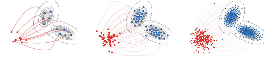
Particle count in the deterministic Wasserstein gradient flow of the squared MMD-type discrepancy to a smooth two-Gaussian teacher distribution, using here the energy-distance kernel $k(x,y)=-\norm{x-y}$. The teacher itself is shown only through true density contours, while red dots are a compact shifted Gaussian initialization placed away from the target, red-to-blue curves show a thinned subset of particle trajectories, and blue dots show the stabilized long-time particles. With too few particles, the empirical measure forms a sparse kernelized quadrature and may under-cover the target modes; increasing $n$ makes the particle cloud approximate the continuous target geometry more faithfully.

The interactive demo turns this finite-particle effect into a parameter: increasing the number of particles makes the same deterministic force field approximate the teacher geometry more faithfully.

show_book_figure("gradflow-interaction-particles")

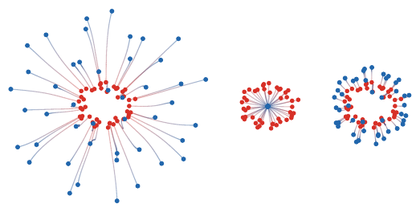
Interaction-energy particle flows for three choices of $k$. A positive Gaussian kernel $k(x,y)=\exp(-\norm{x-y}^2/(2\sigma^2))$ produces short-range repulsion under Wasserstein descent; changing its sign produces attraction and collapse; adding a quadratic long-range attraction to the repulsive kernel yields a balanced attraction--repulsion dynamics. The curves use arclength-based red-to-blue coloring along a longer integration of the coupled particle ODE (20).

The interactive demo lets the sign and strength of the interaction change without editing the hidden particle solver. This is the quickest way to see how the same formal ODE can repel, collapse, or self-organize.

show_book_figure("gradflow-particle-objective-geometries")

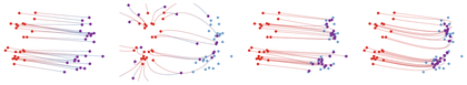
Particle trajectories induced by different discrepancy geometries. The red particles and blue target cloud are the same in all panels. Straight OT displacement produces rays from an optimal matching; an MMD-type witness field gives smoother nonlocal forces; the Sinkhorn-divergence force is an entropic, debiased transport attraction; and the normalized drifting field combines attraction to data with self-repulsion. The figure is qualitative: it compares geometric behavior, not solver performance.

The interactive demo keeps the source and target fixed while switching the discrepancy geometry. The smoothing parameter controls how local or nonlocal the induced force appears.

Stochastic Particles and McKean--Vlasov Limits¶

Deterministic particle flows have stochastic counterparts, where Brownian noise at the particle level becomes an entropy term at the measure level. If the drift does not depend on the empirical measure, each particle evolves independently according to

and the one-particle law $\alpha_t=\rho_t\d x$ satisfies the linear Fokker--Planck equation

For example, if $b=-\nabla V$, this is the $\Wass_2$ gradient flow of the free energy

The mean-field case is different: the drift is recomputed from the current empirical distribution of all particles,

For finite $n$, the empirical law $\mu_t^n$ is random. Under suitable Lipschitz, growth and chaotic-initialization assumptions, propagation of chaos states that finitely many particles become asymptotically independent as $n\to\infty$, all with the same deterministic law $\rho_t\d x$. Equivalently, $\mu_t^n$ converges in probability to this law. The limiting density solves the nonlinear Fokker--Planck, or McKean--Vlasov, equation

When the interaction drift has variational form

this PDE is the Wasserstein gradient flow of the entropy-regularized energy

show_book_figure("gradflow-fokker-planck-three-representations")

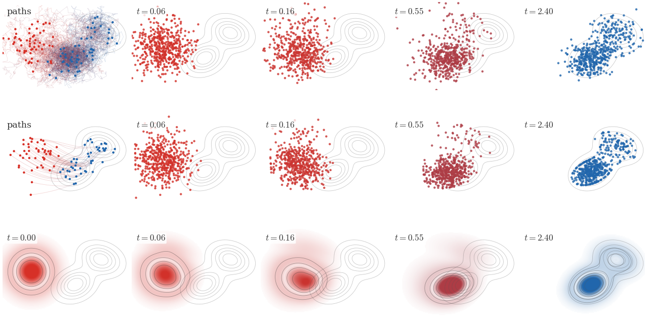
Three numerical representations of the same entropy-regularized Wasserstein gradient flow of $\KL(\rho|\beta)$, where $\beta$ is a two-Gaussian target shifted to the right of an initially isotropic Gaussian density. The first row simulates independent Langevin particles and displays a thinned set of trajectories in the left panel. The second row evolves many deterministic particles with velocity $\tau(\nabla\log\beta-\nabla\log\rho_t)$, estimating $\nabla\log\rho_t$ by a sharper kernel-density score; only representative trajectories and particle subsets are displayed. The third row solves the corresponding Fokker--Planck equation on a grid, starting from the initial density in the left panel. The remaining columns use front-loaded times, so that the onset of the flow and the later deformation toward a bimodal law are both visible.

The interactive demo compares three views of the same entropy-regularized relaxation: stochastic Langevin particles, deterministic score particles, and a smoothed grid density. The noise slider controls the entropy strength.

Geodesic Convexity and Convergence¶

Geodesic convexity is the convexity notion adapted to Wasserstein geometry. It is the condition that turns the formal gradient-flow calculus into a convergence theory.

Geodesics and Convexity¶

A constant-speed $\Wass_2$ geodesic between $\alpha_0$ and $\alpha_1$ is obtained, as in the McCann interpolation, from any optimal coupling $\pi^\star\in\Couplings(\alpha_0,\alpha_1)$ by

where $P_0(x,y)=x$ and $P_1(x,y)=y$. If the optimal plan is induced by a Brenier map $T$, this reduces to $((1-t)\Id+tT)_\sharp\alpha_0$. The coupling formula matters because geodesics exist even when no Monge map exists, for instance when a Dirac mass must split.

Convergence of the Flow¶

In general, analyzing (8) is delicate. The cleanest case is when $f$ is geodesically convex. This condition is the Wasserstein analogue of convexity in Euclidean gradient descent.

Convexity and Curvature¶

The same language is not restricted to subsets of $\RR^d$. If $(\X,\dist,\mathfrak m)$ is a geodesic metric-measure space, $\Wass_2$ geodesics can be defined by transporting each pair of endpoints along metric geodesics, or more intrinsically by dynamical optimal plans on path space. Given a reference measure $\mathfrak m$, the entropy relative to $\mathfrak m$ is

On a smooth Riemannian manifold $(M,g)$, the Ricci curvature tensor $\mathrm{Ric}_g$ is the trace of the Riemann curvature tensor. The lower bound $\mathrm{Ric}_g\geq\lambda g$ means that $\mathrm{Ric}_g(v,v)\geq\lambda |v|_g^2$ for every tangent vector $v$. The fundamental link between curvature and optimal transport is that this tensor lower bound is exactly encoded by geodesic convexity of entropy.

This equivalence was developed in the smooth Riemannian setting by Cordero-Erausquin, McCann and Schmuckenschlaeger and by von Renesse and Sturm Cordero-Erausquin et al., 2001Renesse & Sturm, 2005; it is a central theme of the optimal-transport approach to curvature in Villani’s monograph Villani, 2009. Lott--Villani and Sturm then used the same entropy-convexity principle to define synthetic lower Ricci curvature bounds on metric-measure spaces Lott & Villani, 2009Sturm, 2006Sturm, 2006. Outside this convex, curvature-controlled regime, such as in the mean-field neural-network example below, the flow may still be informative but its convergence analysis requires problem-specific arguments.

Training Two-Layer MLPs as Wasserstein Flows¶

Mean-field limits recast the training of wide neural networks as transport of a distribution of neurons. This section shows how the particle ODE of gradient descent becomes a Wasserstein flow in parameter space.

We use $z\in\RR^d$ for the input data and $y\in\RR^{d'}$ for the label. A neuron is a particle

where $u$ is the inner weight and $v$ is the outer vector weight. For a scalar nonlinearity $\sigma$, define the vector-valued feature

The width-$n$ network and its mean-field version are

This formulation removes the artificial ordering of neurons and allows $\alpha$ to be a continuous distribution of infinitely many neurons.

Let $\rho$ be a probability distribution on data-label pairs $(z,y)\in\RR^d\times\RR^{d'}$. The population risk is

and the empirical risk is the special case $\rho=\rho_N\eqdef N^{-1}\sum_{k=1}^N\delta_{(z_k,y_k)}$. Since $\alpha\mapsto G_\alpha$ is linear, $f$ is convex as a function of $\alpha$ whenever $\ell(\cdot,y)$ is convex. For the empirical neuron law $\alpha_X=n^{-1}\sum_i\delta_{x_i}$, the Wasserstein metric induces on particles the rescaled metric $n^{-1}\sum_i\norm{\dot x_i}^2$. The corresponding particle flow is

This is the gradient flow of $F(X)=f(\alpha_X)$ for the Wasserstein particle metric, equivalently Euclidean gradient descent with time scale multiplied by $n$. It gives a particle discretization of (8).

Assume that $\ell$ is differentiable in its first variable. The first variation is

and the Wasserstein gradient in parameter space is

For the squared Euclidean loss $\ell(s,y)=\frac12\norm{s-y}^2$, the energy is the sum of a quadratic interaction and a linear potential:

with

Thus

These kernels are generally not convex in the particle variable, so the geodesic-convex convergence theory above does not apply directly.

show_book_figure("gradflow-mlp-homogeneous-relu")

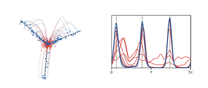
Mean-field training of a homogeneous two-layer model as transport in neuron space. The left panel shows the Wasserstein particle gradient flow in the reduced homogeneous coordinates $(|u|v_1,|u|v_2)$, with black dashed rays marking the teacher directions. The right panel shows the weighted angular density along a front-loaded sequence of times, colored from red to blue, so that the early concentration of neuron directions is visible. The display follows the rendering of the auxiliary MLP experiment but keeps only the $W_2$ flow, not the spectral-flow comparison.

The interactive demo gives a lightweight version of the same phenomenon: particles move in reduced neuron coordinates, while their angles concentrate around the teacher directions.

Classical Convexity and Stationarity¶

Before using the specific homogeneity mechanism of Chizat and Bach, it is useful to isolate a simpler convex-analytic principle behind many mean-field arguments. Consider an energy

on probability measures over a parameter domain. Assume that the quadratic part is convex in the classical affine structure of measures:

This is ordinary convexity of the functional on the convex set of measures, not displacement convexity along $\Wass_2$ geodesics.

The mean-field description of two-layer training was developed in several works, including Chizat & Bach, 2018Mei et al., 2018. The distinctive contribution of Chizat and Bach is a global-convergence analysis for positively homogeneous networks without adding an explicit regularizer or relying on noisy SGD to create a Laplacian term. The following formal statement isolates the core mechanism and ignores the technical issues due to ReLU non-smoothness, support propagation and compactness.