Optimal transport is rarely evaluated on population measures directly. In
machine learning and statistics, the inputs are usually empirical laws,
histograms, simulated particles or minibatches, and the central question is
therefore no longer only how to compute OT, but how OT behaves as a random
estimator. This chapter studies this statistical layer: qualitative consistency
of empirical measures, non-asymptotic sample-complexity rates, and asymptotic
bias--variance decompositions for exact and regularized transport costs.
This statistical convergence is conceptually different from the algorithmic
convergence studied in the previous chapter. There the marginals and the
temperature were fixed and one asked how Sinkhorn iterates approach a
regularized optimizer. Here the number of samples grows, the empirical
measures themselves move, and the regularization parameter may either remain
fixed or be sent to zero. The resulting picture explains why exact OT is
statistically expensive in high intrinsic dimension, why fixed-temperature
Sinkhorn has smoother parametric fluctuations, and why approximating exact OT
with entropy always involves a bias--variance tradeoff.
from pathlib import Path
import sys
from IPython.display import Image as DisplayImage
from IPython.display import display
here = Path.cwd()
myst_dir = None
for candidate in [here, here.parent, here / "myst", here.parent / "myst", here.parent.parent / "myst"]:
if (candidate / "ot4ml_web.py").exists():
myst_dir = candidate.resolve()
sys.path.insert(0, str(myst_dir))
break
if myst_dir is None:
raise RuntimeError("Could not locate myst/ot4ml_web.py")
repo_root = myst_dir.parent
thumbnails = repo_root / "notebooks-figures" / "thumbnails"
def show_book_figure(name, width=760):
display(DisplayImage(filename=str(thumbnails / f"{name}.png"), width=width))
Before discussing sample complexity in Section Sample Complexity, it
is useful to separate consistency from rates. If X1,…,Xn are i.i.d.
samples with common law α, the
associated empirical measure is the random probability measure
The ordinary law of large numbers says that empirical averages converge to
expectations. In measure language this means that α^n converges
weakly toward α, because testing α^n against a bounded
continuous function φ gives the sample average
n−1∑iφ(Xi). Wasserstein distances strengthen this statement by
also recording moment convergence. Thus, if α has a finite p-th
moment, the empirical law converges to α in Wp, almost surely and
in p-th mean in the sense that
EWp(α^n,α)p→0. This is the qualitative consistency
statement behind empirical OT plug-in estimators: empirical transport
distances converge to their population counterparts once the sampled laws
themselves converge in Wasserstein distance. It says nothing yet about the
speed.
Proof
Fix a reference point x0∈X, and write r(x)=d(x,x0). Since X is
Polish, the weak topology on P(X) admits a countable
convergence-determining class (φk)k≥1⊂Cb(X). For each
fixed k, the strong law of large numbers gives
almost surely. Intersecting these probability-one events over the countable set
of indices gives convergence against every φk, hence weak convergence
α^n⇀α.
The moment condition α∈Pp(X) means ∫rpdα<+∞.
Applying the strong law again to r(X1)p gives
almost surely. Weak convergence plus convergence of p-th moments is
equivalent to Wp convergence on Pp(X), so
Wp(α^n,α)→0 almost surely.
For convergence in expectation, set An=∫rpdα^n and
M=∫rpdα. The triangle inequality through the Dirac mass
δx0, followed by (a+b)p≤2p−1(ap+bp), gives
The family (An)n is uniformly integrable. By the de la Vallee--Poussin
criterion, choose a convex superlinear function Ψ such that
EΨ(r(X1)p)<+∞; Jensen’s inequality gives
The previous proposition is a law-of-large-numbers statement: a random
empirical measure converges to the law that generated it. The central limit
theorem describes a different, fluctuation-scale limit. As recalled in Remark
Remark: Central limit theorem, if (Xi)i≥1 are centered i.i.d. random vectors with
identity covariance, the law of n−1/2∑iXi converges weakly toward a
Gaussian. Equivalently, if α is the common law of the Xi, this law is
the rescaled convolution (D1/n)♯α∗n. Wasserstein
distances make this qualitative convergence quantitative. The next result is
a W1 form of the Berry--Esseen theorem: it controls the error uniformly
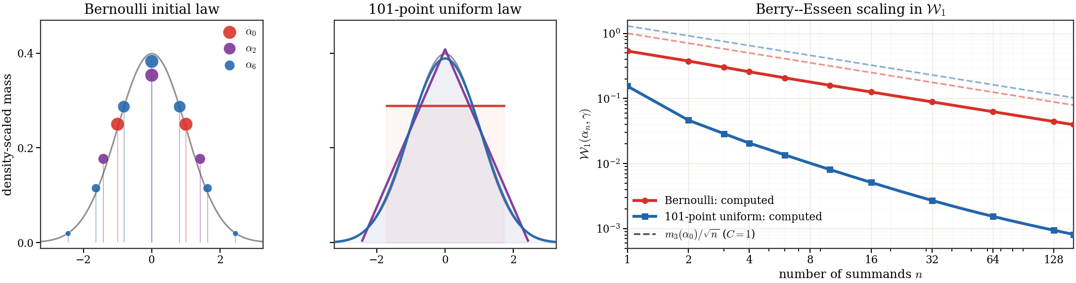
over all 1-Lipschitz test functions. The qualitative Bernoulli example was
visualized earlier in Figure Div.
For each such h, solve Stein’s equation
fh′(x)−xfh(x)=h(x)−Eh(G). Its solution satisfies
∥fh′∥∞+∥fh′′∥∞≤CChen et al., 2011. Writing
Sn(i)=Sn−Xi/n, independence and EXi=0 give
Taylor’s formula with integral remainder and EXi2=1 show that
this differs from n−1∑iEfh′(Sn(i)) by at most
CE∣X1∣3/n. The Lipschitz bound on fh′ replaces this
average by Efh′(Sn) at the same order. Stein’s identity and the
duality formula then prove the claim
Berry, 1941Esseen, 1942Chen et al., 2011Bobkov, 2018Rio, 2011.
The universal n−1/2 bound is sharp over broad classes of input laws, but
it need not describe the asymptotic behavior of a fixed law. For symmetric
inputs, the smooth skewness correction vanishes. What replaces it depends on
whether the law is lattice-valued or has a density.
Proof
Write Fn for the CDF of αn, and Φ and φ for the
standard Gaussian CDF and density. With
ψ(u)=21−{u}, the integrated lattice Edgeworth expansion gives
For completeness, prove this first for compactly supported step functions,
where it is a Riemann sum over periods, and conclude by L1 approximation
of φ.
The absence of a lattice correction reveals the next smooth Edgeworth term.
A density automatically satisfies Cramér’s non-lattice condition because its
characteristic function vanishes at infinity.
Proof
The non-lattice Edgeworth expansion through order n−1 has an
n−1/2 term proportional to the third cumulant, and n−1 terms
proportional to the fourth cumulant and to the square of the third one.
Symmetry makes the third cumulant vanish and gives
These two results explain the different behaviors in Figure
Div. For the symmetric Bernoulli law, the
maximal span is h=2, hence
W1(αn,γ)=1/(2n)+o(n−1/2). The density proposition
cannot be used: this law has no density and its characteristic function is
E[eitX]=cost, whose modulus returns to one at arbitrarily large
frequencies. Thus symmetry removes the smooth skewness term but not the
lattice sawtooth. Conversely, X∼Unif[−3,3] has
a density, characteristic function sin(3t)/(3t)→0, and
κ4=−6/5. Since
so that α1=α. For Bernoulli input, the distance is evaluated by
the exact quantile formula and atom masses are divided by the current lattice
spacing in the density display. For continuous-uniform input, the normalized
convolution is an affine image of the Irwin--Hall distribution, whose density
is, up to rescaling, a cardinal B-spline of degree n−1, and the absolute CDF
difference is integrated numerically. Neither computation uses Monte Carlo
sampling.
Sharp lattice and density central-limit asymptotics in W1. The two
left panels show α1, α2, and α6 for symmetric
Bernoulli and continuous-uniform inputs; the gray curve is the standard
Gaussian density. The right panel compares the exact numerical distances
(solid) with the sharp equivalents in (17)
(dashed). The Bernoulli curve follows its lattice rate 1/(2n), while
the continuous-uniform curve approaches
(1+4e−3/2)/(102πn).
This section compares four statistical regimes. Exact OT resolves geometry at
all scales and pays rates controlled by the intrinsic dimension. MMD replaces
transport by a kernel mean embedding and has a parametric Monte-Carlo rate for
bounded kernels. Fixed-temperature Sinkhorn divergences smooth the dual
potentials and also recover parametric fluctuations, at the price of
regularization bias. Sliced Wasserstein inherits one-dimensional empirical
rates through its projected laws.
The previous section proves qualitative convergence of empirical laws. The
sample-complexity question is how fast this convergence happens. The sample
complexity of unregularized OT suffers from the curse of
dimensionality, but the relevant dimension is geometric. If the distributions
are supported on a regular
lower-dimensional set, for instance a d′-dimensional submanifold of
Rd, the empirical rate is governed by d′ rather than by the ambient
dimension d. In the high-dimensional regime for Wp, namely
d′>2p, this gives the characteristic rate n−1/d′. Exact OT is therefore
dimension-adaptive: it sees the intrinsic dimension of the data support
through its covering numbers Dudley, 1969Weed & Bach, 2019.
Related two-sample-testing viewpoints are developed in
Ramdas et al., 2017.
For n≥2, p≥1, and d≥1, define the worst-case empirical scale
The following proposition turns this scale into uniform one-sample and
two-sample bounds for empirical OT.
The following multiscale estimate makes the mechanism behind the W1
bound explicit.
Proof Sketch
Match the common mass inside the finest cells, then recursively match the
remaining common mass inside each parent cell. Mass first matched at scale
j moves by at most d2−j, and its total amount is bounded by
the sum of the child-cell imbalances. The residual at the finest unresolved
scale has mass at most one and moves by at most d2−J.
Proof of the empirical-OT rate proposition
General empirical Wasserstein moment estimates prove the one-sample statement
for arbitrary pDereich et al., 2013Fournier & Guillin, 2015; reverse
triangle and Minkowski then give the two-sample estimate. We give the direct
multiscale proof for p=1. The triangle inequality reduces the result to
EW1(α^n,α). For each dyadic cell Q,
Optimizing J yields the three displayed regimes for p=1.
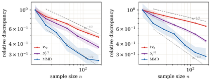
Figure Div gives a numerical overview of these regimes: exact OT exhibits dimension-dependent empirical fluctuations, whereas MMD and fixed-temperature Sinkhorn divergences lie much closer to the parametric n−1/2 scale.
Empirical fluctuations in dimensions three and six. For each sample size
n, two independent empirical measures are drawn from the same standard
Gaussian law. Exact OT follows a slower dimension-dependent scale, while MMD
and the fixed-ϵ Sinkhorn divergence behave closer to the parametric
n−1/2 guide. This is a statistical illustration, not a solver benchmark.
Interactive panel. Vary dimension, sample budget and temperature to compare the curse-of-dimensionality OT guide with the parametric fluctuation and bias floor of entropic OT.
The high-dimensional rate is not merely a defect of the empirical plug-in
estimator. A hypercube of localized density perturbations gives the following
distribution-estimation obstruction
Singh & Póczos, 2018Weed & Bach, 2019Chewi et al., 2025.
Proof Sketch
Partition the cube into M=md cells of width h=1/m, and put an
independent signed, zero-mean bump of fixed small amplitude in each cell.
Kantorovich--Rubinstein duality gives a separation of order
hd+1 per differing sign. Neighboring experiments have one-sample KL
divergence O(hd). Pinsker’s inequality (Theorem: Pinsker Inequality) shows that
choosing M≍n keeps their n-sample total variation bounded away from
one. Assouad’s lemma then gives
Mhd+1=h≍n−1/d.
For a Sobolev-smooth density, convolving the empirical measure at bandwidth
h creates a bias of order hs+1 but reduces the empirical fluctuation to
order n−1/2h1−d/2. Balancing these terms selects
hn≍n−1/(d+2s), which improves on the empirical n−1/d rate
when d>2Niles-Weed & Berthet, 2022Divol, 2022.
Proof Sketch
Kantorovich--Rubinstein duality bounds W1 by the negative Sobolev norm
H˙−1. Since
Eρα~n=ρα∗κh, Fourier estimates
give kernel bias O(hs+1), while Parseval’s identity gives
Balancing the bias with the square root of this fluctuation yields the stated
bandwidth and rate.
The restriction s≤1 permits a nonnegative symmetric kernel and hence a
genuine probability estimator. Exploiting higher smoothness requires
higher-order, generally signed kernels followed by a positivity correction.
Dimensions one and two have separate parametric or logarithmic regimes
Divol, 2022.
This statistical acceleration has a numerical price. For a Gaussian kernel,
α~n is a mixture of n Gaussians, and OT between two such
mixtures has no closed form in general. A direct particle implementation draws
M independent vectors ξi,j∼N(0,Idd) around each
observation and defines
Here addition is understood modulo Zd. Conditionally on the
observations, convexity of W1 under mixing, together with translation,
scaling and the 1-Lipschitz projection onto the torus, gives
The last estimate is the moment form of the empirical OT rate
Fournier & Guillin, 2015. At the optimal bandwidth
hn≍n−1/(d+2s), keeping this extra error below the statistical rate
is guaranteed by
M≳nsd/(d+2s). This componentwise strategy therefore uses
Ncomp=nM≳n1+sd/(d+2s) particles per measure.
Approximating every Gaussian separately is conservative. One can instead
sample or quantize the whole smoothed mixture using N points. In dimension
d>2, the corresponding W1 error is of order N−1/d, up to
dimension-dependent constants Graf & Luschgy, 2000.
Thus target accuracy δ requires N≳δ−d, whereas the
componentwise construction uses
Ncomp≳δ−d−2s/(s+1). The global strategy is cheaper, but
its particle count remains exponential in d at fixed accuracy. Forming and
storing a dense N×N transport kernel costs O(N2) work and memory,
and each direct Sinkhorn scaling costs another O(N2) operations. Fast
kernel summation or low-rank approximations may reduce this matrix cost, but
without additional structure they do not remove the underlying N−1/d
discretization barrier.
MMD contains no transport optimization: its square is a combination of
expectations of kernel evaluations, estimated empirically by sums of kernel
values. Ordinary Monte Carlo averaging therefore gives a dimension-free
parametric rate for bounded kernels. This sharply contrasts with exact
empirical OT, whose value is defined through an optimization problem and whose
worst-case W1 plug-in bias in dimension d>2 decays only as n−1/d,
corresponding to a sample requirement of order δ−d at accuracy
δ. The constants for MMD still depend on the kernel and its bandwidth,
and changing the kernel changes the discrepancy being estimated.
Proof
Let Φ(x)=k(x,⋅) be the feature map and
mα=EΦ(X). The reverse triangle inequality gives
Entropic regularization keeps the transport geometry while smoothing the dual
potentials. The sharp fixed-temperature statement below has polynomial, rather
than exponential, dependence on the inverse temperature
Genevay et al., 2019Mena & Niles-Weed, 2019.
Proof Sketch
Dual optimality bounds a one-marginal perturbation by the empirical process
indexed by normalized entropic potentials. One can show that these potentials
obey polynomial local Hölder bounds under a common subgaussian proxy
Mena & Niles-Weed, 2019.
Their covering numbers have a finite Dudley integral, hence the empirical
process is O(n−1/2) with constant Cd(1+σqd) at
ϵ=1. The rescaling x↦x/ϵ gives the displayed
Λd,σ(ϵ). Perturbing both marginals and applying the
same estimate to the cross and two self terms yields the debiased result.
For fixed ϵ>0, the empirical fluctuation is therefore parametric,
while the prefactor deteriorates only polynomially as ϵ↓0.
Compact support is a special case: if both supports lie in a common ball
B(z,R), translating them by −z leaves the quadratic transport problem
unchanged, and the subgaussian assumption holds with
σ=R/2dlog2=O(R). Genevay--Chizat--Bach--Cuturi--Peyré
established the compactly supported result, and Mena--Niles-Weed extended it to
the subgaussian setting above
Genevay et al., 2019Mena & Niles-Weed, 2019.
The interactive demo below is only a scaling guide: change the dimension to see the
exact-OT exponent flatten, and change ϵ to move the Sinkhorn bias
floor against its parametric fluctuation term.
Interactive panel. This exploratory panel is a scaling guide. Use dimension, sample size, and epsilon to compare statistical fluctuation with regularization bias.
The preceding estimates concern transport values. For map estimation, one
solves the empirical discrete dual problem (2) or its entropic
counterpart (47) for potentials
(fn,mϵ,gn,mϵ)∈Rn×Rm, with
ϵ=0 denoting the unregularized Kantorovich problem, and then uses the
soft c-transform as an out-of-sample extrapolator.
For the quadratic cost c2(x,y)=∥x−y∥2/2, let
Pn,mϵ=(Pijϵ) be the empirical entropic coupling and let
gn,mϵ be the target-side dual potential. Define
Equivalently, subtracting the quadratic marginal terms turns c2 into the
bilinear cost cip(x,y)=−⟨x,y⟩. With the sign convention
used here, the associated soft convex potential is
which is the barycentric projection of the entropic plan. At ϵ=0,
the hard c-transform is generally nondifferentiable: away from Laguerre
boundaries its gradient selects one target site, whereas the barycentric
projection of an optimal unregularized plan may average several target sites
when a row splits. The consistency statement is therefore formulated directly
for barycentric projections. It uses uniform empirical weights; deterministic
nonuniform weights require the corresponding entropy bound.
Proof Sketch
Compare the entropic minimizer with an unregularized empirical optimal plan.
On a uniform n×m grid, this relative entropy is the mutual information
of two uniform indices and is at most min{logn,logm}. Thus the entropic
coupling has asymptotically optimal quadratic cost when
ϵlog(min{n,m})→0. Any weak limit is therefore an optimal population
plan, hence the Brenier graph (Id,T)#α. Jensen’s
inequality applied to each conditional law reduces the claim to the convergence
of ∬∥y−T(x)∥2dPn,mϵ(x,y). This last convergence is
not a continuity tautology, because the Brenier map is only defined
α-a.e. At every differentiability point of ϕ, the subdifferential
is the singleton {∇ϕ(x)}; compactness of the target bounds the
selected subgradients, and the closed-graph property of the subdifferential
then gives continuity of any selected subgradient there. Since convex functions
are differentiable Lebesgue-a.e. and α is absolutely continuous, the
portmanteau theorem for bounded test functions continuous almost everywhere
under the limiting measure gives the desired limit.
Quantitative map convergence requires stronger regularity than consistency.
The following result gives a direct guarantee for the Sinkhorn-based estimator
defined above Pooladian & Niles-Weed, 2021.
This estimator is directly computable from Sinkhorn potentials. Under stronger
modeling and smoothing assumptions, unregularized estimators can attain sharper
minimax rates
Hütter & Rigollet, 2021Deb et al., 2021Manole et al., 2024.
The construction is studied in Sliced Wasserstein Distances. For p=1, it
inherits a particularly clean one-dimensional empirical-CDF rate rather than
an ambient-dimensional matching rate
Nadjahi et al., 2019Nadjahi et al., 2020Manole et al., 2022.
Proof
The triangle inequality reduces the claim to the two one-sample terms
SW1(α^n,α) and SW1(β^m,β). Fix a direction
θ, and let Fθ and F^θ,n be the CDFs of
(Pθ)#α and (Pθ)#α^n. Their supports lie in
[−R,R], and the one-dimensional CDF formula gives
Here nF^θ,n(s) is binomial with success probability
Fθ(s). Integrating over θ yields
ESW1(α^n,α)≤R/n. The same argument for
β concludes the proof.
The previous section answered a coarse but essential question: how many samples
are needed before an empirical OT quantity is accurate, typically up to
universal constants. We now ask for a finer statistical description of the
KL-normalized entropic OT value Lcϵ defined in
(20), with the convention
Lc0:=Lc for unregularized OT. Fixing c, α and β,
define the statistical bias
For the debiased Sinkhorn divergence, define Bˉn,mϵ and
Zˉn,mϵ by replacing Lcϵ with
Lˉcϵ above; the same decomposition then holds with bars. It is
usually read after choosing a temperature ϵ=ϵn. At fixed
ϵ>0 and on finite supports, the statistical bias is typically
O(n−1+m−1), while the centered fluctuation is
OP(n−1/2+m−1/2). The regularization bias disappears only
when ϵ→0, whereas the fluctuation constants can deteriorate in this
limit. This is the bias--variance tradeoff illustrated in
Div.
The remainder of this section analyzes the latter two terms. The superscript
records their dependence on the regularization strength. The empirical
fluctuation is pushed through the nonlinear transport value Lcϵ,
which can be nonsmooth at ϵ=0. Its limiting law is governed by local
differentiability and by the geometry of the optimal dual potentials.
For exact OT on finite spaces, empirical central-limit theorems follow from a
directional delta method Sommerfeld & Munk, 2018Tameling et al., 2019;
fixed positive entropic regularization makes the transport value smooth on the
interiors of the marginal simplices
Bigot et al., 2019Klatt et al., 2020Hundrieser et al., 2021Mena & Niles-Weed, 2019.
The following statement isolates the Gaussian regime common to both settings:
at zero temperature, uniqueness of the dual potentials turns the directional
derivative into an ordinary linear derivative.
Proof
Writing a^n and b^n for the two empirical histograms, the
independent multinomial central-limit theorems give
where Ga and Gb are independent centered Gaussian vectors with covariance
matrices diag(a)−aa⊤ and
diag(b)−bb⊤. Proposition
Proposition: First variations of OT values gives the directional derivative
for every ϵ≥0. It is linear under the assumed uniqueness at
ϵ=0, and automatically at positive temperature. Thus,
The delta method therefore gives the Gaussian limit
∑ifϵ⋆(xi)(Ga)i+∑jgϵ⋆(yj)(Gb)j. Independence and the two multinomial
covariance formulas give exactly vϵ.
It remains to justify convergence of the moments, which does not follow from
convergence in distribution alone. Set
R=maxi,jc(xi,yj)−mini,jc(xi,yj). Exact dual potentials may be
replaced by their c-transforms, and entropic potentials by their soft
c-transforms; in either case their oscillations are at most R. Since
differences of histograms have zero sum, integrating the corresponding
subgradient bounds along segments in the two marginal simplices gives, for any
histograms (a′,b′) and their associated measures (α′,β′),
Because N,M are fixed, the fourth moments of
n∥a^n−a∥1 and n∥b^n−b∥1 are uniformly
bounded. The squared rescaled OT values are therefore uniformly integrable.
The Gaussian limit then yields convergence of the means and second moments,
which proves the assertions for Bn,nϵ, Zn,nϵ, and the
variance.
For fixed ϵ>0, the entropic value is twice continuously differentiable
in a neighborhood of the positive pair (a,b). A second-order Taylor expansion
on this neighborhood has a uniformly bounded remainder; its linear term has
zero expectation and
E(∥a^n−a∥2+∥b^n−b∥2)=O(n−1). The probability
of leaving the neighborhood is exponentially small, and the preceding global
Lipschitz bound controls its contribution. Hence
Bn,nϵ=O(n−1).
The uniqueness assumption at ϵ=0 is substantive. Without it, the
directional delta method gives the generally non-Gaussian limit
where Dc(α,β) is the set of optimal dual pairs modulo the
additive gauge. Its expectation need not vanish, so the exact-OT bias can then
have order n−1/2 rather than being negligible at the central-limit scale
Sommerfeld & Munk, 2018Tameling et al., 2019.
The variance does not necessarily diverge with N,M: for a uniformly bounded
cost, normalized dual potentials have bounded oscillation, hence
vϵ remains bounded. What fails to be uniform is the
differentiability argument. If amin=miniai and
bmin=minjbj, then
P[some source or target atom is unobserved]≤Ne−namin+Me−nbmin.
For nearly uniform weights, making this probability vanish already requires
both n≫NlogN and n≫MlogM. Moreover, exact-dual uniqueness margins can
close as the supports become dense, while entropic Hessian bounds can
deteriorate with the smallest weights and as ϵ↓0. Thus the
constant hidden in the bias estimate may grow even when the first-order
variance stays bounded.
There is therefore no distribution-free passage from this multinomial CLT to
arbitrary continuous laws. Continuous CLTs nevertheless hold under hypotheses
ensuring stable unique potentials, with limiting variance
Varα(fϵ⋆)+Varβ(gϵ⋆)
in the independent two-sample setting
Barrio & Loubes, 2019Barrio et al., 2021Mena & Niles-Weed, 2019González-Sanz & Hundrieser, 2023.
The first-order description ceases to be informative in degenerate regimes. For
instance, when ϵ=0, c=dp, and α=β, the first
derivative vanishes; the two-sample empirical cost
Ldp(α^n,β^n) is instead governed by the
dimension-dependent matching behavior studied in Sample Complexity.
This is where the curse of dimensionality re-enters. The first derivative of
the debiased Sinkhorn divergence also vanishes under the null, so its nontrivial
limit is of second order
Goldfeld et al., 2024.
The statistical results above explain why entropic OT is attractive at fixed
temperature, but they also expose a computational tension. Sampling the
marginals replaces the input laws by empirical measures and reduces the problem
to finitely many support points; subsampling or coarsening these supports is
governed by the sample-complexity estimates of this chapter. Even after the
supports are fixed, however, a Sinkhorn sweep still costs O(nm), because it
repeatedly applies the Gibbs kernel to vectors. Kernel sketching attacks this
second bottleneck: it keeps the sampled marginals fixed and samples, or
otherwise compresses, the feature representation of the kernel used by
Sinkhorn. With a rank R factorization, Nit scaling sweeps cost
O(Nit(n+m)R), which is linear in the support sizes only when both the
required rank and the iteration count are controlled. The rank generally
depends on dimension, temperature, and target accuracy.
The RKHS/MMD section, Dual RKHS Norms and Maximum Mean Discrepancies, already used positive semidefinite
kernels to define Hilbertian discrepancies between measures. Recall that a
symmetric kernel k:X×X→R is positive semidefinite if, for every
finite family (xi)i=1n, the Gram matrix (k(xi,xj))ij is positive
semidefinite. Many scalable kernel methods start from an integral feature
representation
This is the classical random-feature principle. Given two point families
(xi)i=1n and (yj)j=1m, define the rectangular cross-kernel matrix
K∈Rn×m by Kij=k(xi,yj). Set R=rp, flatten
(ℓ,q) into a single feature index, and define
Although K is generally rectangular and hence is not itself a Gram matrix,
it is a cross-block of the Gram matrix evaluated on the union of the two point
families. When the families coincide, ΦX=ΦY=Φ, and the construction
reduces to the symmetric approximation K=ΦΦ⊤. The number
r of sampled latent variables is thus a second sample size, distinct from n
and m. At this stage no positivity of ϕ is assumed; signed or oscillatory
features are exactly what make Fourier sketches useful.
For translation-invariant kernels on Rd, Bochner’s theorem gives the
standard Fourier sketch. If k(x,y)=κ(x−y) and
κ(t)=∫ei⟨ω,t⟩dΛ(ω), with Λ a
positive spectral measure, one may use real features
ϕ(x,ω)=(cos⟨ω,x⟩,sin⟨ω,x⟩). For the Gaussian
kernel kσ(x,y)=exp(−∥x−y∥2/(2σ2)), this corresponds to
ω∼N(0,σ−2Id). This random Fourier feature
construction was introduced by Rahimi and Recht to accelerate large-scale
kernel machines Rahimi & Recht, 2007; its statistical role
for kernel ridge regression and related supervised methods is analyzed, for
instance, in
Rudi & Rosasco, 2017Avron et al., 2017.
The following concentration bound assesses the entrywise quality of the
rectangular sketch (69). This is the relevant
control when the kernel will subsequently be used inside logarithms or
componentwise divisions.
Proof
For each fixed (i,j), the summands in the definition of
Kij have expectation Kij and lie in [−M,M].
Hoeffding’s inequality therefore gives
A union bound over the nm entries proves
(72). On its complementary
event, write Kij=Kij(1+sij), where
∣sij∣≤δ≤1/2. Hence Kij>0, and
∣log(1+sij)∣≤2∣sij∣ gives the logarithmic estimate.
Specialize the preceding construction to the Gibbs kernel
kϵ(x,y)=e−c(x,y)/ϵ, assumed to be PSD and to admit the
displayed feature representation. Thus the rectangular matrix defined above is
precisely the Sinkhorn kernel, Kij=kϵ(xi,yj). Assume that the
weights and the entries of K are positive. Recall the Sinkhorn scaling
equations (8):
so each scaling sweep costs O((n+m)R) operations and stores only
O((n+m)R) numbers. The difficulty is that Sinkhorn is not a generic kernel
method: it divides by Kv and, in dual variables, applies
logarithms. Thus one needs Kij>0, preferably with a relative
error on the entries, because −ϵlogKij is the effective cost.
This is a more stringent requirement than the usual spectral or Frobenius
approximation of a PSD Gram matrix.
The interaction between kernel accuracy and scaling accuracy can be quantified
for Gaussian kernels. The following specialization of the Nyström--Sinkhorn
analysis of Altschuler, Bach, Rudi and Niles-Weed
Altschuler et al., 2018Altschuler et al., 2019
uses ϵ for the entropic temperature and τ for the requested
numerical accuracy. We write O for bounds up to logarithmic factors
in N, 1/τ, and 1/δ.
Proof
Apply the Gaussian Nyström approximation to the Gram matrix on the union of the
N support points and retain its source--target block. Since
∥x−y∥≤2D, one has Kmin≥e−4D2/ϵ. The adaptive
stopping rule of Altschuler, Bach, Rudi and Niles-Weed resolves the kernel below
this scale, hence produces K>0 with the same logarithmic control
singled out in Proposition: Entrywise Accuracy of Rectangular Feature Sketches. Their Gaussian
effective-dimension estimate gives (79).
Stability of entropic OT with respect to logK, followed by approximate
Sinkhorn scaling and rounding, gives the two error bounds. The low-rank
factorization costs O(NR2) to construct, each kernel product costs O(NR),
and the quantitative scaling bound contributes
O(NRD4/(ϵτ)), yielding the stated time and memory
estimates. Their entropy convention differs from the KL-normalized value
Lcϵ only by a constant depending on (a,b), so the approximation
bounds are unchanged.
The power d in (79) is the principal
limitation. Sinkhorn requires K>0 and control of
logK, so an additive kernel approximation must resolve entries as
small as e−4D2/ϵ. The Gaussian effective dimension at this
resolution scales as (D2/ϵ)d, up to logarithmic factors. For example,
when n=m and both measures are uniform,
0≤Lcϵ−Lc≤ϵlogn. Approximating unregularized OT
to accuracy τ therefore calls for ϵ of order τ/logn, and
the sufficient rank scales as τ−d up to powers of D and logarithmic
factors. This is the dimension-dependent price of the sketch; replacing d by
a smaller intrinsic dimension is possible under additional geometric
assumptions on the data
Altschuler et al., 2019.
The preceding analysis identifies positivity as a central bottleneck: a signed
sketch may require many features merely to avoid negative entries, whereas
Sinkhorn repeatedly divides by kernel--vector products and therefore cannot
tolerate this failure. A natural remedy is to build entrywise nonnegativity
into every sketch by using nonnegative features; under a mild nondegeneracy
condition, the resulting entries are strictly positive. Not every positive
semidefinite and pointwise-positive kernel admits such a representation,
however. We therefore first identify the matrix and kernel classes for which
positive sketches are possible. In finite dimension, let
DNNn={A∈Rn×n:A⪰0,Aij≥0},CPn={BB⊤:B∈R+n×q for some q≥1}.
Matrices in DNNn are doubly nonnegative, while matrices in
CPn are completely positive. One always has
CPn⊂DNNn, with equality for n≤4 and strict
inclusion for n≥5Berman & Shaked-Monderer, 2003Burer et al., 2009. Thus, from five
sampled points onward, positive sketchability is strictly more demanding than
being doubly nonnegative: the latter is the spectral and entrywise positivity
condition desirable for stable Sinkhorn kernels, whereas the former guarantees
nonnegative low-rank features and hence positive Sinkhorn sketches. This gap
does not occur for ordinary sketches, where no sign constraint is imposed on
the features: spectral positivity is equivalent to the existence of a possibly
signed Hilbert feature representation. It appears only when one insists that
every feature, and hence every finite sketch, be pointwise nonnegative. Checking
membership in the completely positive cone is computationally hard: strong
membership is NP-hard, and weak membership for the completely positive cone and
its copositive dual is NP-hard Dickinson & Gijben, 2014.
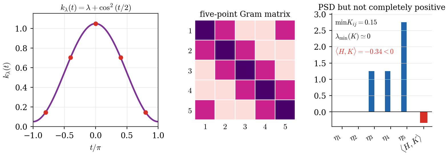
A concrete five-point obstruction is provided by the periodic kernel
It is PSD and strictly positive pointwise because
cos2(t/2)=(1+cost)/2 has nonnegative Fourier coefficients. Yet, for
λ=1/20, its Gram matrix K on five equally spaced points is not
completely positive. Indeed, the Horn copositive matrix H is nonnegative on
CP5, whereas
The integrand belongs to the closed convex cone CPn, hence so does
K.
The zero kernel is trivial. Otherwise, choose a dk-dense sequence (xi)
and positive weights (ωi) such that
0<S:=∑iωik(xi,xi)<+∞. Factor each
finite Gram matrix as K(r)=B(r)(B(r))⊤. If bℓ are its
nonzero columns, set
tℓ=∑i≤rωi(bℓ)i2,
Sr=∑ℓtℓ, and
zi(r,ℓ)=Sr/tℓ(bℓ)i for i≤r, with zero
coordinates afterward. The probability measures
are supported on the compact product
∏i[0,S/ωi] and satisfy
∫zizjdξr=k(xi,xj) for i,j≤r. A weak limit ξ gives
scalar nonnegative features ϕ(xi,z)=zi. Their L2(ξ)-distance is
dk(xi,xj), so they extend by continuity to all x∈X, remain
nonnegative, and have inner products k(x,y).
The separability assumption holds for continuous kernels on separable metric
spaces. It cannot be omitted for a common probability feature space: the delta
kernel on an uncountable discrete set has completely positive finite Gram
matrices but would require uncountably many pairwise orthogonal nonzero
elements of L+2(ξ). For a rectangular source--target matrix, the
proposition is applied to the Gram matrix on the union of the two point sets,
after which one extracts the rectangular cross block.
Despite this certification difficulty, completely positive kernels,
equivalently positive-sketchable kernels under the preceding proposition,
enjoy a useful closure algebra. It provides a systematic way to construct new
kernels whose low-rank features remain nonnegative.
Proof
On an arbitrary finite point set, nonnegative sums are handled by concatenating
nonnegative factors. If Kj=BjBj⊤, then
so pointwise products are completely positive. Measurable nonnegative mixtures
remain in the closed convex cone CPn. The autocorrelation formula
is directly a scalar positive-feature representation, so the same integral
argument applies.
For the quadratic cost c(x,y)=∥x−y∥2, the Gaussian Gibbs kernel used
by Sinkhorn admits an especially simple positive feature representation,
which is the construction exploited by Scetbon and Cuturi
Scetbon & Cuturi, 2020. The same construction extends to
the generalized Gaussian kernels
e−∥x−y∥p/ϵ for 0<p≤2, because these kernels are
mixtures of Gaussian kernels. This is the Schoenberg--Bernstein mechanism
behind the positive definiteness of radial stable kernels
Schoenberg, 1938Berg et al., 1984.
The factor 1/p, often used in the definition of Wpp, only rescales
ϵ. For p≥1, this is the usual p-Wasserstein power cost; for
0<p<1, it should be read simply as a concave power transport cost.
Using the sketching features φℓ of Proposition
Proposition: Generalized Gaussian Positive Features, define directly
The proposition gives Kr:=ΦXΦY⊤≥0 entrywise and
E[Kr]=K. Sinkhorn applied to Kr uses only products by the two
feature matrices, and its plan is represented as
This route is complementary to
worst-case near-linear Sinkhorn analyses Altschuler et al., 2017, low-rank
Gaussian-kernel approximations for quadratic transport
Altschuler et al., 2018, and factored-coupling
models in which the coupling itself is constrained to have low rank
Scetbon et al., 2021.
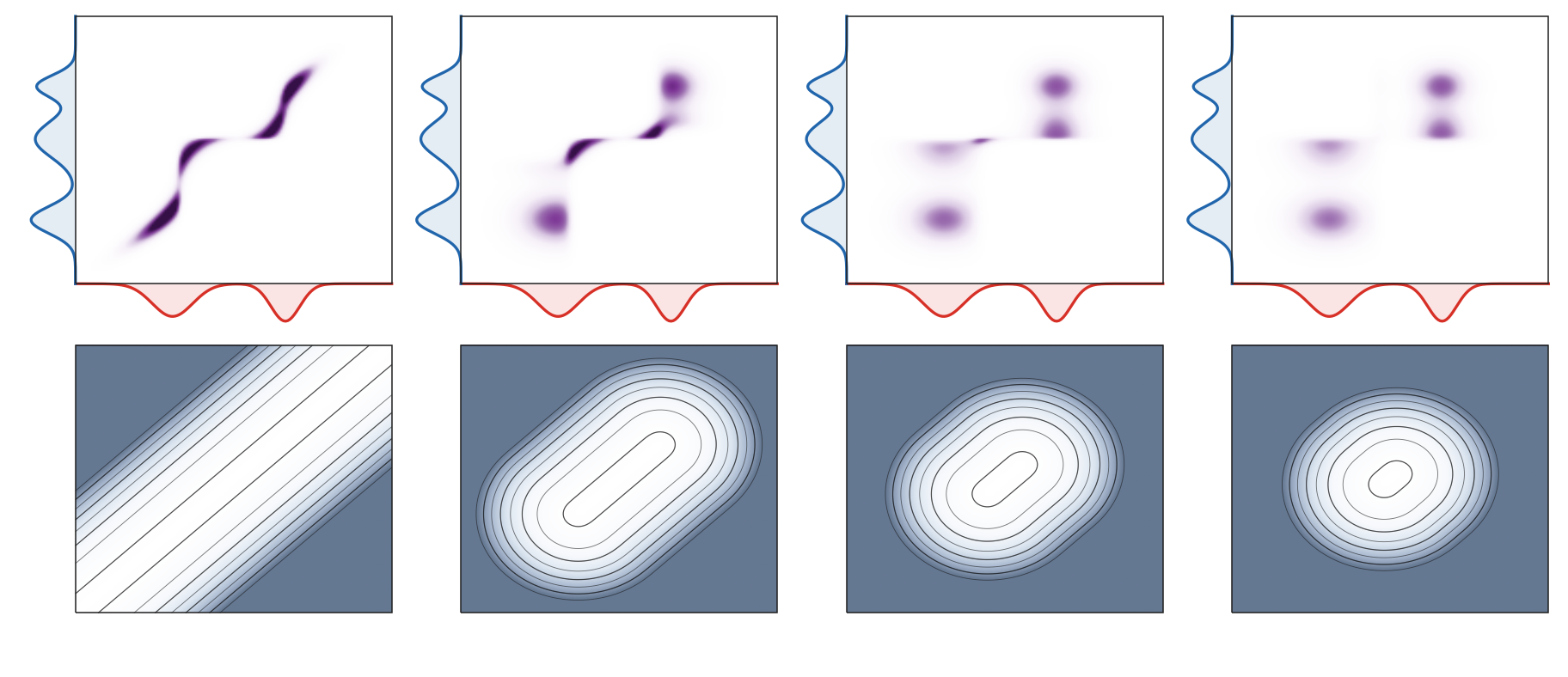
Figure Notebook-code uses the p=2 Gaussian
Gibbs kernel. A sufficiently large rank gives a visually accurate plan and
entrywise logarithm of the kernel matrix, whereas coarse sketches preserve the
marginals but lose geometric concentration.
The top row shows the entropic couplings. The bottom row displays the entries
−ϵlog(Kr)i,j with black level sets, compared with the exact
quadratic cost ∣xi−yj∣2 in the first column. Rank 40 remains close to the dense
computation, while ranks 10 and 3 preserve the marginals but increasingly
blur the transport geometry.
Interactive panel. Change the regularization and random seed to compare the
exact Gibbs matrix with positive low-rank sketches and their logarithmic
matrices.
The same algebra appears in transformer attention, studied later from a
continuous-depth transport viewpoint in
Evolution in Depth of Transformers. A softmax attention matrix has entries
proportional to exp(⟨qi,kj⟩); linear-attention methods
replace this positive kernel by features Φ(qi)⊤Φ(kj), so that
attention can be applied as Φ(Q)(Φ(K)⊤V) rather than by forming
the full n×n matrix
Katharopoulos et al., 2020Choromanski et al., 2021Wang et al., 2020Xiong et al., 2021.
Sinkhorn sketching is the transport analogue of this idea: replace the Gibbs
matrix by a positive feature factorization, keep only the scaling vectors and
feature factors, and control the approximation in the logarithmic scale
relevant to entropic potentials. The transport case is more constrained,
however, since the approximate kernel is reused inside nonlinear normalizations
until the prescribed marginals are reached for the sketched problem.
Chen, L. H. Y., Goldstein, L., & Shao, Q.-M. (2011). Normal Approximation by Stein’s Method. Springer.
Berry, A. C. (1941). The Accuracy of the Gaussian Approximation to the Sum of Independent Variates. Transactions of the American Mathematical Society, 49(1), 122–136.
Esseen, C.-G. (1942). On the Liapunoff Limit of Error in the Theory of Probability. Arkiv for Matematik, Astronomi Och Fysik, 28A(9), 1–19.
Bobkov, S. G. (2018). Berry–Esseen bounds and Edgeworth expansions in the central limit theorem for transport distances. Probability Theory and Related Fields, 170, 229–262.
Rio, E. (2011). Asymptotic constants for minimal distance in the central limit theorem. Electronic Communications in Probability, 16, 96–103.
Petrov, V. V. (1975). Sums of Independent Random Variables (Vol. 82). Springer-Verlag. 10.1007/978-3-642-65809-9
Bhattacharya, R. N., & Ranga Rao, R. (2010). Normal Approximation and Asymptotic Expansions (Vol. 64). Society for Industrial. 10.1137/1.9780898719895
Kolassa, J. E., & McCullagh, P. (1990). Edgeworth Series for Lattice Distributions. The Annals of Statistics, 18(2), 981–985. 10.1214/aos/1176347637
Vallender, S. S. (1974). Calculation of the Wasserstein Distance Between Probability Distributions on the Line. Theory of Probability and Its Applications, 18(4), 784–786. 10.1137/1118101
Dudley, R. M. (1969). The speed of mean Glivenko-Cantelli convergence. Annals of Mathematical Statistics, 40(1), 40–50.
Weed, J., & Bach, F. (2019). Sharp asymptotic and finite-sample rates of convergence of empirical measures in Wasserstein distance. Bernoulli, 25(4A), 2620–2648. 10.3150/18-BEJ1065
Ramdas, A., Trillos, N. G., & Cuturi, M. (2017). On Wasserstein two-sample testing and related families of nonparametric tests. Entropy, 19(2), 47.
Dereich, S., Scheutzow, M., & Schottstedt, R. (2013). Constructive quantization: Approximation by empirical measures. Annales de l’Institut Henri Poincaré, Probabilités et Statistiques, 49(4), 1183–1203.
Fournier, N., & Guillin, A. (2015). On the rate of convergence in Wasserstein distance of the empirical measure. Probability Theory and Related Fields, 162(3–4), 707–738.
Singh, S., & Póczos, B. (2018). Minimax Distribution Estimation in Wasserstein Distance. arXiv Preprint arXiv:1802.08855. https://arxiv.org/abs/1802.08855