Entropic Regularization: Convergence

Convergence for entropic optimal transport has two complementary meanings. At fixed marginals and fixed temperature, one studies how Sinkhorn iterates approach the regularized optimizer. When the marginals are empirical, one also studies how the regularized value and potentials behave as the number of samples grows toward a mean-field limit.

This chapter keeps these two scales together. It starts with algorithmic convergence of matrix scaling and soft transforms, then explains the Hilbert metric contraction mechanism, and finally turns to Gaussian closed forms and sample-complexity consequences. The recurring message is that entropy helps optimization and statistics by smoothing the problem, but the constants deteriorate as the temperature $\epsilon$ goes to zero.

from pathlib import Path
import sys

from IPython.display import Image as DisplayImage
from IPython.display import display

here = Path.cwd()
myst_dir = None
for candidate in [here, here.parent, here / "myst", here.parent / "myst", here.parent.parent / "myst"]:
    if (candidate / "ot4ml_web.py").exists():
        myst_dir = candidate.resolve()
        sys.path.insert(0, str(myst_dir))
        break

if myst_dir is None:
    raise RuntimeError("Could not locate myst/ot4ml_web.py")

repo_root = myst_dir.parent
thumbnails = repo_root / "notebooks-figures" / "thumbnails"

def show_book_figure(name, width=760):
    display(DisplayImage(filename=str(thumbnails / f"{name}.png"), width=width))

Sinkhorn Convergence: Bregman View¶

Sinkhorn can be read as alternating Bregman projections. The main geometric message is simple: each row or column rescaling is the KL projection onto one affine marginal constraint. The convergence mechanism then follows from the Pythagorean identity for Bregman divergences.

For simplicity, this section is written for discrete measures. The same ideas carry over to general measures, and the robust-rate section below expresses the constants through cost and potential oscillations rather than through the number of grid points.

Alternating KL Projections¶

The projection viewpoint explains Sinkhorn as repeated enforcement of one marginal constraint at a time. It is not specific to entropy, although KL is the case where the projections reduce to elementary row and column scalings.

Bregman divergences are useful because their geometry can encode constraints. A Legendre-type generator blows up, or has an infinite derivative, at the boundary of its domain. For negative entropy, positivity is therefore built into the divergence, so one projects onto affine marginal constraints without separately handling non-negativity.

Linear Tilts and Gibbs References¶

Adding a linear cost to a Bregman penalty merely shifts the reference point in dual coordinates. The usual Gibbs--KL reformulation is exactly the entropy specialization.

For the negative entropy, take $Q=a\otimes b$ . The tilted reference is

K_{a,b}^\epsilon \eqdef (a\otimes b)\odot e^{-C/\epsilon}.

(5)

Thus

\langle P,C\rangle+\epsilon\operatorname{KL}(P\mid a\otimes b) = \epsilon\operatorname{KL}(P\mid K_{a,b}^\epsilon)+\text{cst}.

(6)

On the transport polytope, scaling $K_{a,b}^\epsilon$ is equivalent to scaling the Gibbs kernel $K=e^{-C/\epsilon}$ because the factors $a_i$ and $b_j$ can be absorbed into the Sinkhorn scalings. The unique entropic optimizer is the KL projection of this tilted Gibbs reference onto the coupling constraints:

P_\epsilon = \argmin_{P\in\mathcal U(a,b)} \operatorname{KL}(P\mid K_{a,b}^\epsilon).

(7)

Cyclic Projection Convergence¶

The convergence mechanism is the classical one of Bregman projections Bregman, 1967.

Proposition: Cyclic Bregman Projections on Affine Constraints

Let $\Phi$ be a Legendre strictly convex generator on a finite-dimensional convex domain, and let $\mathcal C_1,\mathcal C_2$ be affine constraint sets whose intersection meets the domain. Define

P_{k+1} = \operatorname{Proj}_{\mathcal C_2}^{B_\Phi} \operatorname{Proj}_{\mathcal C_1}^{B_\Phi}(P_k),

(8)

starting from an interior point $P_0$ . Assume the projections are well-defined and the iterates remain in a compact subset of the domain. Then $P_k$ converges to the Bregman projection of $P_0$ onto $\mathcal C_1\cap\mathcal C_2$ . In particular, the KL case converges for positive affine marginal constraints on a bounded transportation polytope.

Let

\mathcal C_a^1 \eqdef \{P:P\mathbf 1_m=a\}, \qquad \mathcal C_b^2 \eqdef \{P:P^\top\mathbf 1_n=b\}.

(11)

Then $\mathcal U(a,b)=\mathcal C_a^1\cap\mathcal C_b^2$ , and KL cyclic projections read

P^{(2\ell+1)} = \operatorname{Proj}_{\mathcal C_a^1}^{\operatorname{KL}}(P^{(2\ell)}), \qquad P^{(2\ell+2)} = \operatorname{Proj}_{\mathcal C_b^2}^{\operatorname{KL}}(P^{(2\ell+1)}).

(12)

The preceding proposition applies with $P_0=K_{a,b}^\epsilon$ and gives convergence to the entropic optimizer.

Row and Column Scalings¶

The projectors are explicit because they only rescale rows or columns.

Defining

P^{(2\ell)} \eqdef \operatorname{diag}(u^{(\ell)})K\operatorname{diag}(v^{(\ell)}),

(15)

the two projection steps are the usual Sinkhorn updates on the scaling vectors. In practice one stores the vectors and multiplies by the Gibbs kernel, often exploiting separable, sparse, low-rank or geometric structure.

The Bregman proof is geometric, but its direct finite-dimensional linear-rate constants can degrade with dimension and with small $\epsilon$ . The robust dual analysis below gives a dimension-free qualitative message: before any local linear regime becomes visible, one can still guarantee an $O(1/k)$ dual gap whose constants depend on the cost range and potential oscillation.

Algorithm: Cyclic Bregman projections

Input: Constraint sets $\Cc_1,\Cc_2$ , Bregman divergence $B_\Phi$ , interior point $P_0$ , constraint defects $\mathrm{def}_{\Cc_1},\mathrm{def}_{\Cc_2}$ , tolerance $\mathrm{tol}$ .

Output: Point in $\Cc_1\cap\Cc_2$ when the intersection is feasible.

Specialize to entropic OT, if needed: $\Cc_1=\Cc^1_\a, \qquad \Cc_2=\Cc^2_\b, \qquad B_\Phi=\KL.$

Initialize: Set $r_0=+\infty$ and $k=0$ .

While $r_k>\mathrm{tol}$ do:

Set $k\leftarrow k+1$ .
$P_{k-1/2}=\Proj_{\Cc_1}^{B_\Phi}(P_{k-1}).$
$P_k=\Proj_{\Cc_2}^{B_\Phi}(P_{k-1/2}).$
Set $r_k=\max\{\mathrm{def}_{\Cc_1}(P_k),\mathrm{def}_{\Cc_2}(P_k)\}$ .

Return $P_k$ .

Sinkhorn Convergence: Monotone Point of View¶

There is another, older route to convergence, going back to Fortet’s proof of the Schrodinger system Fortet, 1940Essid & Pavon, 2019Léonard, 2019. It uses the order structure of soft transforms rather than an explicit contraction factor.

Proposition: Monotone Fixed-Point Route to Sinkhorn Convergence

Let $c$ be bounded and continuous on compact spaces, and define the double Sinkhorn map, normalized by subtracting its $\alpha$ -mean,

\mathcal A(f) \eqdef (f^{c,\epsilon})^{\bar c,\epsilon} - \int (f^{c,\epsilon})^{\bar c,\epsilon}\,\d\alpha .

(16)

The map $\mathcal A$ is order preserving on the quotient by additive constants. If a representative of the initial class is chosen so that $f_0\leq\mathcal A(f_0)$ , then representatives of the iterates $f_{k+1}=\mathcal A(f_k)$ can be chosen to increase pointwise, remain uniformly bounded in oscillation, and converge to a fixed point. Since constants are free, any bounded initialization can be shifted downward to satisfy the subsolution inequality. The fixed point is the entropic potential, hence the associated Sinkhorn scalings converge.

This proof is qualitative rather than quantitative, but it is conceptually useful: Sinkhorn is not only alternating projection or projective contraction; it is also a monotone fixed-point iteration on potential classes once constants are quotiented out.

This is the natural size for Sinkhorn potentials because adding constants changes their gauge but not the coupling.

Sinkhorn Convergence: Sublinear Robust Rate¶

Sinkhorn is cyclic coordinate ascent on the smooth dual objective; equivalently, it alternates KL projections on the two marginal constraint sets. The rate most useful for complexity estimates is the pre-asymptotic one: before a linear regime becomes visible, the dual objective gap decreases at order $1/k$ . Related robust Bregman-projection rates are developed in Peyré, 2026Altschuler et al., 2017Dvurechensky et al., 2018, and statistical consequences of entropic smoothing in Genevay et al., 2019Bigot et al., 2019.

Corollary: Approximating Unregularized OT by Regularized Dual Costs

Consider histograms $a\in\simplex_n$ , $b\in\simplex_m$ and a finite cost matrix $C$ . Let $\mathcal D_{\epsilon,k}$ be the KL-normalized entropic dual value after $k$ Sinkhorn cycles, and let $\Delta_k$ be its dual gap. Define the entropy-corrected lower bound

L_{\epsilon,k} \eqdef \mathcal D_{\epsilon,k} - \epsilon H(a) - \epsilon H(b), \qquad H(a)=-\sum_i a_i\log a_i .

(31)

Then

0 \leq \operatorname{OT}_C(a,b)-L_{\epsilon,k} \leq \epsilon\log(nm)+\Delta_k .

(32)

Thus, choosing $\epsilon\leq\delta/(2\log(nm))$ and running Sinkhorn until $\Delta_k\leq\delta/2$ gives a $\delta$ -accurate lower bound on the unregularized OT value. Under the compact $O(1/k)$ rate, it is sufficient to take

k+1 \geq \frac{4 C R^2\log(nm)}{\delta^2},

(33)

up to constants and logarithmic stabilization factors.

The same identity yields computable stopping diagnostics. The KL drops are exactly marginal defects: after a row update the row marginal is correct and the remaining drop is measured by the column marginal, and conversely after a column update. Marginal violations therefore monitor both feasibility and the remaining dual gap, up to the bounded-radius constant.

Algorithm: Certified entropic approximation of discrete OT

Input: Cost matrix $C\in\RR^{n\times m}$ , weights $\a,\b$ , target accuracy $\delta>0$ .

Output: Certified lower bound $L_{\epsilon,k}$ for exact OT.

Set $\epsilon=\frac{\delta}{2\log(nm)}.$

Initialize stabilized Sinkhorn potentials and set $k=0$ , $\widehat\Delta_0=+\infty$ .

While $\widehat\Delta_k>\delta/2$ do:

Set $k\leftarrow k+1$ .
Compute one row soft-transform update and one column soft-transform update in stabilized log-domain variables.
Compute the entropic dual value $\mathcal D_{\epsilon,k}$ and the certified gap upper bound $\widehat\Delta_k$ .

Return $L_{\epsilon,k} = \mathcal D_{\epsilon,k} - \epsilon\HD(\a)-\epsilon\HD(\b), \qquad 0\leq\MKD_{\C}(\a,\b)-L_{\epsilon,k}\leq\delta.$

Sinkhorn Convergence: Linear Hilbert Metric Rate¶

Hilbert’s projective metric gives a complementary convergence mechanism. Instead of following objective values, it measures distances between positive scaling vectors modulo global multiplication. Positive kernels are contractions in this geometry, yielding a global linear convergence statement Franklin & Lorenz, 1989.

Multiplying both vectors by arbitrary positive constants does not change this quantity, so it is a distance only after passing to projective classes.

Hilbert’s metric was introduced by Birkhoff and Samelson to give quantitative proofs of the Perron--Frobenius theorem Birkhoff, 1957Samelson, 1957. Sinkhorn can be viewed as a nonlinear matrix-scaling analogue of this theory.

Theorem: Linear Convergence of Sinkhorn

Let $(u^{(\ell)},v^{(\ell)})$ be Sinkhorn scaling iterates and $(u^\star,v^\star)$ optimal scalings. Then

\mathsf H(u^{(\ell)},u^\star)=O(\lambda(K)^{2\ell}), \qquad \mathsf H(v^{(\ell)},v^\star)=O(\lambda(K)^{2\ell}).

(40)

Moreover, for $P^{(\ell)}=\operatorname{diag}(u^{(\ell)})K\operatorname{diag}(v^{(\ell)})$ ,

\mathsf H(u^{(\ell)},u^\star) \leq \frac{\mathsf H(P^{(\ell)}\mathbf 1_m,a)}{1-\lambda(K)}, \qquad \mathsf H(v^{(\ell)},v^\star) \leq \frac{\mathsf H((P^{(\ell)})^\top\mathbf 1_n,b)}{1-\lambda(K)}.

(41)

The primal logarithmic error satisfies

\norm{\log P^{(\ell)}-\log P^\star}_\infty \leq \mathsf H(u^{(\ell)},u^\star)+\mathsf H(v^{(\ell)},v^\star).

(42)

For bounded cost, the contraction can also be read directly on the dual potentials. With $K_\epsilon=e^{-c/\epsilon}$ and $R=\sup c-\inf c$ ,

\lambda(K_\epsilon) \leq \tanh(R/(2\epsilon)).

(44)

This is a useful global statement, but it also explains a limitation: the worst-case factor becomes exponentially close to one as $\epsilon\to0$ . In practice, one often observes a much better local linear regime after enough iterations. The same Hilbert-metric mechanism extends beyond finite matrices to positive integral operators under compactness and positivity assumptions, but Gaussian distributions with quadratic cost require a different approach.

The interactive demo below separates the observed marginal residual from two theoretical guides. The $O(1/k)$ curve captures the robust pre-asymptotic message, while the Hilbert curve shows how pessimistic the global contraction bound becomes when the Gibbs kernel is close to degenerate.

Interactive panel. This exploratory panel plots convergence guides for Sinkhorn iterations. Use epsilon and condition controls to compare observed residuals with pessimistic global contraction bounds.

Entropic Optimal Transport Between Gaussians¶

Gaussian marginals provide an explicit finite-dimensional model of Sinkhorn’s behavior. The soft $c$ -transform preserves quadratic potentials, the optimal entropic coupling is Gaussian, and the value can be written with matrix square roots Janati et al., 2020. This is the entropic counterpart of the Gaussian $\Wass_2$ and Bures formula.

Proposition: Quadratic Closure of Sinkhorn Iterates

Let $\beta=\mathcal N(m_\beta,\Sigma_\beta)$ on $\RR^d$ and take $c(x,y)=\norm{x-y}^2$ . If $g(y)$ is a quadratic polynomial such that the Gaussian integral below is finite, then the soft transform

f(x) = -\epsilon\log \int \exp\!\left(\frac{g(y)-\norm{x-y}^2}{\epsilon}\right) \,\d\beta(y)

(45)

is a quadratic polynomial in $x$ . In particular, starting Sinkhorn from $g_0=0$ gives

f_1(x) = \frac{\epsilon}{2} \log\det\!\left(I+\frac{2\Sigma_\beta}{\epsilon}\right) + \epsilon \left\langle x-m_\beta, (\epsilon I+2\Sigma_\beta)^{-1}(x-m_\beta) \right\rangle .

(46)

Proposition: Balanced Entropic OT Between Gaussians

Let $\alpha=\mathcal N(m_\alpha,\Sigma_\alpha)$ and $\beta=\mathcal N(m_\beta,\Sigma_\beta)$ with positive-definite covariances, and let

\Sigma_\alpha^{1/2}\Sigma_\beta^{1/2} = U\operatorname{diag}(\sigma_i)V^\top

(47)

be a singular-value decomposition. For the balanced objective

\min_{\pi\in\Couplings(\alpha,\beta)} \int\norm{x-y}^2\,\d\pi(x,y) + \epsilon\operatorname{KL}(\pi\mid\alpha\otimes\beta),

(48)

the optimizer is Gaussian with cross-covariance

K_\epsilon = \Sigma_\alpha^{1/2} U\operatorname{diag}(s_i)V^\top \Sigma_\beta^{1/2}, \qquad s_i = \frac{\sqrt{\epsilon^2+16\sigma_i^2}-\epsilon}{4\sigma_i}.

(49)

The optimal value is

\norm{m_\alpha-m_\beta}^2 + \operatorname{tr}(\Sigma_\alpha) + \operatorname{tr}(\Sigma_\beta) + \sum_i \left( -2\sigma_i s_i - \frac{\epsilon}{2}\log(1-s_i^2) \right).

(50)

As $\epsilon\downarrow0$ , $s_i\to1$ and the full covariance contribution converges to the Bures--Wasserstein covariance term.

Corollary: Gaussian Sinkhorn Divergence and Smoothed Bures Term

For $r>0$ , define

\tau_\epsilon(r) \eqdef \frac{\sqrt{\epsilon^2+16r^2}-\epsilon}{4r}, \qquad \psi_\epsilon(r) \eqdef -2r\,\tau_\epsilon(r) - \frac{\epsilon}{2}\log(1-\tau_\epsilon(r)^2).

(53)

If $\sigma_i(\Sigma,\Lambda)$ denotes the singular values of $\Sigma^{1/2}\Lambda^{1/2}$ and $\lambda_i(\Sigma)$ the eigenvalues of $\Sigma$ , then the debiased Gaussian Sinkhorn divergence is

\overline{\mathcal L}_{\norm{\cdot-\cdot}^2}^{\epsilon}(\alpha,\beta) = \norm{m_\alpha-m_\beta}^2 + \mathcal B_\epsilon(\Sigma_\alpha,\Sigma_\beta)^2,

(54)

where

\mathcal B_\epsilon(\Sigma,\Lambda)^2 \eqdef \sum_i\psi_\epsilon(\sigma_i(\Sigma,\Lambda)) - \frac12\sum_i\psi_\epsilon(\lambda_i(\Sigma)) - \frac12\sum_i\psi_\epsilon(\lambda_i(\Lambda)).

(55)

Moreover $\mathcal B_\epsilon(\Sigma,\Lambda)^2\to \mathcal B(\Sigma,\Lambda)^2$ as $\epsilon\downarrow0$ .

The controls below expose exactly the quantities in the formula: $\epsilon$ sets the singular-value shrinkage, anisotropy changes the eigenvalues, and the angle changes the covariance misalignment.

Interactive panel. This exploratory panel exposes the Gaussian formula directly. Use epsilon, anisotropy, and angle to see how entropic shrinkage changes the covariance term.

Proposition: One-Dimensional Gaussian Sinkhorn Rate

Consider $\alpha=\beta=\mathcal N(0,1)$ on $\RR$ with $c(x,y)=(x-y)^2$ . If a dual potential has the form $g_q(y)=q y^2+\text{cst}$ , then one soft transform has quadratic coefficient

T_\epsilon(q) = 1-\frac{1}{1-q+\epsilon/2}, \qquad q<1+\epsilon/2.

(58)

One full Sinkhorn cycle acts as $q\mapsto T_\epsilon(T_\epsilon(q))$ . The fixed point $q_\star=T_\epsilon(q_\star)$ is determined by

A_\star^2-\frac{\epsilon}{2}A_\star-1=0, \qquad A_\star \eqdef 1-q_\star+\frac{\epsilon}{2} = \frac{\epsilon+\sqrt{\epsilon^2+16}}{4}.

(59)

Consequently the local asymptotic contraction factor of one full Sinkhorn cycle on the quadratic coefficient is

\rho_\epsilon = A_\star^{-4} = \left(\frac{4}{\epsilon+\sqrt{\epsilon^2+16}}\right)^4 .

(60)

This scalar calculation illustrates the general Gaussian convergence picture of Chizat, Delalande and Vaskevicius Chizat et al., 2024: the rate improves when $\epsilon$ is large or the covariance scales overlap well, and deteriorates in the small-temperature limit where the entropic coupling approaches a deterministic Brenier map.

Algorithm: Closed-form Gaussian Sinkhorn coupling

Input: Gaussian marginals $\al=\Gaussian(\mean_\al,\cov_\al)$ , $\be=\Gaussian(\mean_\be,\cov_\be)$ , scale $\epsilon>0$ .

Output: Gaussian entropic coupling covariance.

Compute singular value decomposition $\cov_\al^{1/2}\cov_\be^{1/2} = U\diag(\sigma_i)V^\top .$

For each $\sigma_i>0$ do

$s_i=\frac{\sqrt{\epsilon^2+16\sigma_i^2}-\epsilon}{4\sigma_i}.$

Set cross-covariance: $K_\epsilon = \cov_\al^{1/2}U\diag(s_i)V^\top\cov_\be^{1/2}.$ Return Gaussian coupling with means $(\mean_\al,\mean_\be)$ , marginal covariances $(\cov_\al,\cov_\be)$ , and cross-covariance $K_\epsilon$ .

Sample Complexity¶

This section separates two statistical regimes. Exact OT resolves geometry at all spatial scales and pays dimension-dependent empirical rates. Fixed temperature Sinkhorn divergences smooth the dual potentials and recover parametric fluctuations, at the price of regularization bias.

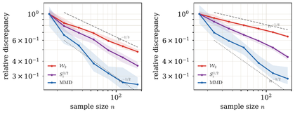
The sample complexity of unregularized OT suffers from the curse of dimensionality. Entropic regularization changes the picture: for a fixed $\epsilon>0$ , Sinkhorn divergences have parametric $n^{-1/2}$ statistical rates, although the constant deteriorates when $\epsilon\to0$ Genevay et al., 2019Bigot et al., 2019. Related two-sample-testing viewpoints are developed in Ramdas et al., 2017, and the large- $\epsilon$ kernel limit connects to classical MMD tests Gretton et al., 2012.

Empirical fluctuations in dimensions three and six. For each sample size $n$ , two independent empirical measures are drawn from the same standard Gaussian law. Exact OT follows a slower dimension-dependent scale, while MMD and the fixed- $\epsilon$ Sinkhorn divergence behave closer to the parametric $n^{-1/2}$ guide. This is a statistical illustration, not a solver benchmark.

Proposition: MMD has a Parametric Value Rate

Let $k$ be a bounded positive definite kernel with RKHS $\mathcal H_k$ , and define

\operatorname{MMD}_k(\alpha,\beta) \eqdef \norm{ \int k(x,\cdot)\,\d(\alpha-\beta)(x) }_{\mathcal H_k}.

(66)

If $\hat\alpha_n$ and $\hat\beta_m$ are independent empirical measures, then

\mathbb E \abs{ \operatorname{MMD}_k(\hat\alpha_n,\hat\beta_m) - \operatorname{MMD}_k(\alpha,\beta) } \leq \kappa\left(\frac1{\sqrt n}+\frac1{\sqrt m}\right)

(67)

when $k(x,x)\leq\kappa^2$ .

Proposition: Sinkhorn Divergences Interpolate the Rates

Assume $\alpha$ and $\beta$ are supported in a compact subset of $\RR^d$ and the cost is smooth. For fixed $\epsilon>0$ , debiased Sinkhorn divergences satisfy representative empirical bounds of the form

\mathbb E \abs{ \overline{\mathcal L}_c^\epsilon(\hat\alpha_n,\hat\beta_m) - \overline{\mathcal L}_c^\epsilon(\alpha,\beta) } \leq C_{c,d}\epsilon^{-d/2} \left( \frac1{\sqrt n}+\frac1{\sqrt m} \right),

(70)

up to constants and exponents depending on the precise smoothness class and support diameter. Thus regularization removes the $n^{-1/d}$ curse for fixed $\epsilon$ , while the prefactor deteriorates as $\epsilon\to0$ .

Remark: No free lunch when approximating exact OT

The parametric rate in Proposition Proposition: Sinkhorn Divergences Interpolate the Rates holds for fixed $\epsilon$ . If the goal is to approximate the unregularized OT value, one must also account for the regularization bias. In a typical bounded-cost finite-dimensional regime,

\abs{\bar\MK_\c^\epsilon(\alpha,\beta)-\MK_\c(\alpha,\beta)} \leq C\epsilon, \qquad \EE\abs{\bar\MK_\c^\epsilon(\hat\alpha_n,\hat\beta_n)-\bar\MK_\c^\epsilon(\alpha,\beta)} \leq C_{c,d}\epsilon^{-d/2}n^{-1/2}.

(71)

Balancing the two terms gives $\epsilon\simeq n^{-1/(d+2)}$ and total error of order $n^{-1/(d+2)}$ . Equivalently, target accuracy $\eta$ requires choosing $\epsilon\simeq\eta$ and $n\simeq\eta^{-(d+2)}$ samples under this bound. Thus entropic smoothing improves the statistical behavior at fixed scale, but approximating exact OT still forces a bias-variance tradeoff whose exponent deteriorates with dimension.

The interactive demo below is only a scaling guide: change the dimension to see the exact-OT exponent flatten, and change $\epsilon$ to move the Sinkhorn bias floor against its parametric fluctuation term.

Interactive panel. This exploratory panel is a scaling guide. Use dimension, sample size, and epsilon to compare statistical fluctuation with regularization bias.

References¶

Bregman, L. M. (1967). The relaxation method of finding the common point of convex sets and its application to the solution of problems in convex programming. USSR Computational Mathematics and Mathematical Physics, 7(3), 200–217.
Fortet, R. (1940). Résolution d’un système d’équations de M. Schrödinger. Journal de Mathématiques Pures et Appliquées, 19(1–4), 83–105. https://www.numdam.org/item/JMPA_1940_9_19_1-4_83_0/
Essid, M., & Pavon, M. (2019). Traversing the Schrödinger Bridge Strait: Robert Fortet’s Marvelous Proof Redux. Journal of Optimization Theory and Applications, 181, 23–60.
Léonard, C. (2019). Revisiting Fortet’s proof of existence of a solution to the Schrödinger system. arXiv Preprint arXiv:1904.13211.
Lemmens, B., & Nussbaum, R. (2012). Nonlinear Perron-Frobenius Theory (Vol. 189). Cambridge University Press.
Peyré, G. (2026). Robust Sublinear Convergence Rates for Iterative Bregman Projections. arXiv Preprint arXiv:2602.01372.
Altschuler, J., Weed, J., & Rigollet, P. (2017). Near-linear time approximation algorithms for optimal transport via Sinkhorn iteration. Advances in Neural Information Processing Systems, 30, 1964–1974.
Dvurechensky, P., Gasnikov, A., & Kroshnin, A. (2018). Computational Optimal Transport: Complexity by Accelerated Gradient Descent Is Better Than by Sinkhorn’s Algorithm. In J. Dy & A. Krause (Eds.), Proceedings of the 35th International Conference on Machine Learning (Vol. 80, pp. 1367–1376). PMLR.
Genevay, A., Chizat, L., Bach, F., Cuturi, M., & Peyré, G. (2019). Sample Complexity of Sinkhorn Divergences. Proceedings of the Twenty-Second International Conference on Artificial Intelligence and Statistics, 89, 1574–1583.
Bigot, J., Cazelles, E., & Papadakis, N. (2019). Central limit theorems for entropy-regularized optimal transport on finite spaces and statistical applications. Electronic Journal of Statistics, 13(2), 5120–5150. 10.1214/19-EJS1637
Franklin, J., & Lorenz, J. (1989). On the scaling of multidimensional matrices. Linear Algebra and Its Applications, 114, 717–735.
Birkhoff, G. (1957). Extensions of Jentzsch’s theorem. Transactions of the American Mathematical Society, 85(1), 219–227.
Samelson, H. (1957). On the Perron-Frobenius theorem. Michigan Mathematical Journal, 4(1), 57–59.
Janati, H., Muzellec, B., Peyré, G., & Cuturi, M. (2020). Entropic Optimal Transport between Unbalanced Gaussian Measures has a Closed Form. Advances in Neural Information Processing Systems.
Chizat, L., Delalande, A., & Vaškevičius, T. (2024). Sharper Exponential Convergence Rates for Sinkhorn’s Algorithm in Continuous Settings. arXiv Preprint arXiv:2407.01202.