Generalized Wasserstein Distances

The first family of extensions keeps the idea of a distance between measures, but changes the geometry used to compare them. The variants in this chapter relax mass conservation, reduce high-dimensional transport to one-dimensional projections, or replace the trace quadratic cost by spectral gauges and robust projected viewpoints.

These constructions are useful when the standard distance $\Wass_p$ is too rigid or too expensive. They preserve much of the metric intuition of optimal transport, but expose new controls: how expensive it is to delete mass, which projections should be trusted, and which directions of displacement should be penalized.

from pathlib import Path
import sys

from IPython.display import Image as DisplayImage
from IPython.display import display

here = Path.cwd()
myst_dir = None
for candidate in [here, here.parent, here / "myst", here.parent / "myst", here.parent.parent / "myst"]:
    if (candidate / "ot4ml_web.py").exists():
        myst_dir = candidate.resolve()
        sys.path.insert(0, str(myst_dir))
        break

if myst_dir is None:
    raise RuntimeError("Could not locate myst/ot4ml_web.py")

repo_root = myst_dir.parent
thumbnails = repo_root / "notebooks-figures" / "thumbnails"

def show_book_figure(name, width=760):
    display(DisplayImage(filename=str(thumbnails / f"{name}.png"), width=width))

Unbalanced OT¶

Unbalanced OT allows mass creation and destruction by penalizing marginal mismatch. It is essential when histograms are not normalized, when observations contain outliers, or when only part of the source should match the target Liero et al., 2018Chizat et al., 2018Chizat et al., 2018.

Relaxed Formulation¶

For nonnegative measures $(\alpha,\beta)\in\mathcal M_+(\X)\times\mathcal M_+(\Y)$, a generic relaxed formulation is

where $\psi_1,\psi_2$ are convex entropy functions. Exact conservation $(\pi_1,\pi_2)=(\alpha,\beta)$ is replaced by a cost for changing the marginals. Writing $\psi_s=\tau\bar\psi_s$ exposes the relaxation scale:

Large $\tau$ makes marginal mismatch expensive and approaches balanced OT when the total masses are compatible. Small $\tau$ makes creation and destruction cheap; after rescaling by $\tau$, the zero-transport part reveals the pure divergence geometry.

Reverse and Homogeneous Formulations¶

The Liero--Mielke--Savare formulation rewrites marginal penalties as a local transport cost and then homogenizes it. Assuming first that the reference measures and transported marginals have mutually absolutely continuous parts, one can factor the objective as

This motivates the local reverse cost

with the usual recession convention at $r=0$ or $s=0$. If $\alpha=F\pi_1+\alpha^\perp$ and $\beta=G\pi_2+\beta^\perp$ are the Lebesgue decompositions of the reference marginals with respect to the transported marginals, then

The homogeneous formulation is obtained by taking the perspective transform of $L_c$,

which is positively 1-homogeneous. It defines

Conic Lifting¶

Assume now that $\X=\Y$ and $\psi_1=\psi_2=\psi$. The homogeneous formulation lifts the problem to the cone space $\mathfrak C[\X]\eqdef(\X\times\RR_+)/\sim$, where all points $(x,0)$ are identified at the apex. For an exponent $p\geq1$, define

Several classical unbalanced geometries are obtained by choosing $\psi$, $c$ and $p$ so that $\mathsf D$ is a distance on the cone:

• $\mathcal D_\psi=\operatorname{KL}$, $p=2$, and $c(x,y)=-\log\cos^2(d(x,y)\wedge\pi/2)$ give the Hellinger--Kantorovich or Wasserstein--Fisher--Rao cone metric

• $\mathcal D_\psi=\operatorname{KL}$, $p=2$, and $c(x,y)=d(x,y)^2$ give the Gaussian Hellinger cone metric

• $\mathcal D_\psi=\TV$, $p=1$, and $c(x,y)=d(x,y)$ give the partial-transport cone cost

The corresponding cone value is

Entropic KL Relaxation¶

A generic entropic regularization of unbalanced OT reads

Its dual is

For $\mathcal D_\phi=\operatorname{KL}$, the primal-dual relation is $\d\pi=e^{(f\oplus g-c)/\epsilon}\d\alpha\d\beta$. If in addition $\mathcal D_{\psi_1}=\mathcal D_{\psi_2}=\tau\operatorname{KL}$, coordinate maximization gives the damped soft transforms

In the discrete case, with $K_{i,j}=e^{-C_{i,j}/\epsilon}a_i b_j$ and $\rho=\tau/(\tau+\epsilon)$, this gives the generalized Sinkhorn scaling

The exponent $\rho<1$ is the visible difference with balanced Sinkhorn: marginal corrections are damped because violating the marginals is allowed.

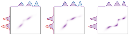
show_book_figure("unbalanced-mass-relaxation")

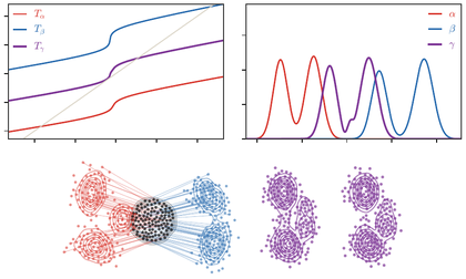
KL unbalanced OT on one-dimensional Gaussian-mixture densities. The central matrix is the transported coupling. The side curves compare the prescribed marginals with the transported marginals; increasing $\tau$ makes marginal mismatch more expensive, so more mass is moved rather than created or destroyed.

The interactive demo below exposes the two most important regularization scales. Increasing $\tau$ pushes the transported marginals closer to the prescribed ones; increasing $\epsilon$ spreads the coupling itself.

The entropy used in the marginal relaxation also changes the qualitative behavior. A KL penalty leads to smooth multiplicative rescaling. The reverse-KL, or Burg, penalty blows up when a transported marginal vanishes where the prescribed marginal is positive, so it discourages complete deletion of small modes. Total variation has a linear kink and behaves closer to partial transport: mass is either kept active or created and destroyed at nearly constant marginal price.

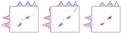
show_book_figure("unbalanced-divergence-choice")

Effect of the marginal divergence in unbalanced entropic OT. The geometric cost, entropic plan regularization $\epsilon$, and relaxation strength $\tau$ are fixed; only the marginal penalty changes. KL allows smooth mass variation, Burg keeps transported marginals from vanishing on prescribed modes, and total variation gives a sharper active-mass selection.

Sliced Wasserstein Distances¶

Sliced Wasserstein trades exact high-dimensional geometry for many one-dimensional projections. It is cheap, differentiable after sorting, and often effective in imaging and learning. For measures on $\RR^d$ and $\theta\in\mathbb S^{d-1}$, let $P_\theta(x)=\dotp{\theta}{x}$ be the projection on direction $\theta$.

This construction is closely related to the Radon transform and is much cheaper to approximate numerically than high-dimensional OT, since each projected problem can be solved by sorting or quantiles Rabin et al., 2011Bonneel et al., 2015Kolouri et al., 2016. It metrizes the same weak-plus-moment topology as $\Wass_p$, but its geometry is not bi-Lipschitz equivalent to $\Wass_p$ in high dimension Nadjahi et al., 2019.

show_book_figure("sliced-wasserstein-projections")

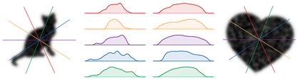
Sliced Wasserstein projections between two planar densities. Fixed directions are drawn on both densities, and the middle panels show smoothed one-dimensional density estimates of the projected measures. Sliced OT averages one-dimensional Wasserstein discrepancies over many such directions.

The interactive demo separates two uses of a slice: comparing projected measures and lifting the sorted one-dimensional matching back to the plane. The lifted plan is always feasible in the original space, but it need not be the quadratic optimal plan.

Subspace-Sliced Variants¶

One-dimensional slices are extremely cheap, but they may discard too much geometry in high dimension. A natural compromise is to project onto $k$-dimensional subspaces: the projected OT problems remain lower dimensional, while each projection retains correlations inside a small block of coordinates.

Min-Sliced Lifted Transport Plans¶

The preceding constructions define distances between projected measures. A different use of slicing is to use a projection only as a device for building a feasible high-dimensional transport plan. For equal-weight empirical measures $\alpha=n^{-1}\sum_i\delta_{x_i}$ and $\beta=n^{-1}\sum_i\delta_{y_i}$, sort the projected samples $\dotp{x_i}{\theta}$ and $\dotp{y_j}{\theta}$, and let $\sigma_\theta$ be the monotone matching induced by this sorting. The lifted plan

is a genuine coupling between $\alpha$ and $\beta$ in the original space. Min-SWGG-type methods then choose the projection whose lifted plan has the smallest full-dimensional quadratic cost:

This quantity is not a projected distance; it is a cheap feasible-plan construction. Consequently,

show_book_figure("min-sliced-transport-plan")

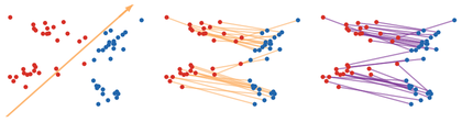
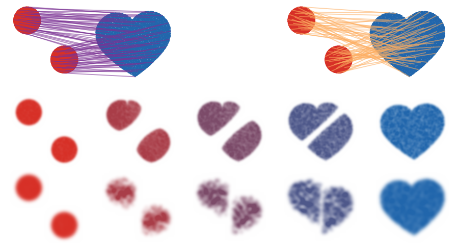
Lifted min-sliced plan. A one-dimensional direction is selected by a small deterministic sweep, then red and blue atoms are sorted after projection and matched in that order. The middle panel lifts this one-dimensional matching back to the plane; it is a feasible coupling but not the same object as the quadratic $W_2$ matching shown on the right.

Vector Quantiles and Linear Optimal Transport¶

Linear OT starts from the multivariate analogue of quantile coordinates. The one-dimensional quantile function represents a probability measure by the monotone map sending a fixed reference law to it; in dimension $d>1$, Brenier’s theorem gives the corresponding construction after choosing an absolutely continuous reference probability $\rho$, typically the uniform law on a convex body or a standard Gaussian.

Vector Quantiles¶

Assume that $\rho$ is absolutely continuous. For a target law $\mu$ with finite second moment, its vector quantile relative to $\rho$ is the Brenier map

or equivalently the solution of

This construction is canonical only after fixing $\rho$: changing the reference law changes the coordinates used to represent $\mu$. Vector quantile regression uses the same idea conditionally, replacing scalar conditional quantiles by conditional Brenier maps and thereby encoding multivariate ranks and depths Carlier et al., 2017.

Linearized Wasserstein Coordinates¶

Linear OT replaces a nonlinear transport distance by a Hilbert norm between reference maps. It is useful when one reference measure is fixed and many nearby distributions must be compared cheaply. Let $T_\alpha$ be the Brenier map pushing $\rho$ to $\alpha$, understood as an element of $L^2(\rho;\RR^d)$ and hence defined only $\rho$-almost everywhere. The linear OT embedding is

If one of the two targets equals the reference, the linearized distance is exact: for instance, $\operatorname{LOT}_\rho(\rho,\alpha) =\norm{T_\alpha-\Id}_{L^2(\rho)} =\Wass_2(\rho,\alpha)$. For two arbitrary targets, the coupling $(T_\alpha,T_\beta)_\sharp\rho$ is admissible but not generally optimal, so $\operatorname{LOT}_\rho$ is a tangent-space approximation of the Wasserstein geometry Wang et al., 2013.

For a family $(\alpha_s)_s$ with weights $(\lambda_s)_s$, the linearized barycenter is obtained by averaging maps,

This is exact in one dimension, where quantile functions linearize $\Wass_2$, and it is especially useful when many barycenters with changing weights must be evaluated quickly.

show_book_figure("dualnorms-linear-ot-embedding")

Linear OT coordinates. Fixing a reference measure $\rho$ turns each target into a map $T_\alpha$ from $\rho$ to $\alpha$, or equivalently into the displacement field $T_\alpha-\Id$. In one dimension this is exactly the quantile parametrization of $\Wass_2$. In two dimensions, averaging the maps gives the linearized barycenter, which is compared with the genuine McCann midpoint.

The next control keeps the exact one-dimensional setting. The reference density defines the coordinate system, the target maps are quantile maps from that reference, and the barycenter is obtained by averaging those maps before pushing the reference forward.

Spectral and Robust Wasserstein Distances¶

Spectral OT changes the scalar quadratic cost by measuring the whole displacement covariance through a matrix gauge. The same object admits a robust projected formulation: instead of fixing one projection, one maximizes over the polar set of the gauge. Subspace robust OT is the important non-convex rank-constrained version of this idea Paty & Cuturi, 2019; spectral gauges provide its convex minimax counterpart and connect to recent spectral-gradient viewpoints such as Muon dynamics Peyré, 2026.

The monotonicity condition means that increasing the displacement covariance in Loewner order cannot decrease the transport penalty.

The special case $\gamma(M)=\tr(M)$ gives the usual quadratic Wasserstein distance $\Wass_2$. The spectral gauge $\gamma(M)=\lambda_{\max}(M)$ instead measures the worst transported variance direction. For $A\succeq0$, define the quadratic projected transport cost

The polar set of the gauge is

so that, for a closed gauge, $\gamma(M)=\sup_{A\in\mathcal B_\gamma}\tr(AM)$.

For the Ky Fan gauge

where the eigenvalues are sorted in decreasing order, the polar set is

Thus $k=d$ gives $\gamma_d(M)=\tr(M)$ and recovers $\Wass_2$. The convex hull of rank-$k$ projectors is

and, since $M\succeq0$, the associated support function is the same Ky Fan gauge. Thus $\Wass_{\gamma_k}$ is the convexified spectral counterpart of $\operatorname{SRW}_{2,k}$, while $\operatorname{SRW}_{2,k}$ keeps the original non-convex rank constraint. For $k=1$, $\gamma_1(M)=\lambda_{\max}(M)$ and $\mathcal B_{\gamma_1}=\{A\succeq0:\tr(A)\leq1\}$.

show_book_figure("spectral-wasserstein-gauge")

Trace and spectral gauges for displacement covariances. The trace gauge minimizes the average squared displacement and gives the usual quadratic transport plan. The $\lambda_{\max}$ gauge penalizes the worst projected displacement variance; the displayed plan is obtained by approximating the robust formulation with finitely many directions.

The interactive demo turns the displacement covariance into a visible object. The trace gauge sums both covariance eigenvalues, while the top-eigenvalue gauge cares only about the worst transported direction.