Generalized OT Problems

The second family changes the optimization problem rather than only the ground distance. Barycenters average several measures, multi-marginal OT couples many measures at once, inverse OT learns the cost from observed transport, and weak OT allows randomized conditional responses.

These formulations remain close to Kantorovich linear programming, but the object being optimized is richer than a single two-marginal coupling.

from pathlib import Path
import sys

from IPython.display import Image as DisplayImage
from IPython.display import display

here = Path.cwd()
myst_dir = None
for candidate in [here, here.parent, here / "myst", here.parent / "myst", here.parent.parent / "myst"]:
    if (candidate / "ot4ml_web.py").exists():
        myst_dir = candidate.resolve()
        sys.path.insert(0, str(myst_dir))
        break

if myst_dir is None:
    raise RuntimeError("Could not locate myst/ot4ml_web.py")

repo_root = myst_dir.parent
thumbnails = repo_root / "notebooks-figures" / "thumbnails"

def show_book_figure(name, width=760):
    display(DisplayImage(filename=str(thumbnails / f"{name}.png"), width=width))

OT Barycenters¶

Barycenters ask how to average probability measures rather than points. This section explains the variational definition, the special closed forms in one dimension and for Gaussians, and the entropic algorithms used in practice.

Frechet Means¶

For discrete input histograms $\{b_s\}_{s=1}^S$, with $b_s\in\simplex_{n_s}$, and weights $\lambda\in\simplex_S$, a Wasserstein barycenter can be computed by minimizing

where the cost matrices $C_s\in\RR^{n\times n_s}$ are prescribed. This barycenter problem was introduced by Carlier and coauthors, following earlier matching ideas, and is the measure-valued analogue of a Frechet mean Agueh & Carlier, 2011Carlier & Ekeland, 2010.

Given input measures $(\beta_s)_s$ on a space $\X$, the barycenter problem is

For $\X=\RR^d$ and $c(x,y)=\norm{x-y}^2$, if one input measure has a density, then the barycenter is unique Agueh & Carlier, 2011. Discrete existence, consistency, and fixed-point constructions are studied in Anderes et al., 2016Esteban et al., 2016Le Gouic & Loubes, 2016.

show_book_figure("barycenters-four-shapes")

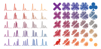
Wasserstein barycenter grids for four corner measures. The left panel uses the one-dimensional formula $Q_{u,v}=\sum_{i,j}\lambda_{ij}(u,v)Q_{ij}$ for one Gaussian law and three asymmetric two-Gaussian mixtures, and displays densities reconstructed from the averaged quantiles. The right panel computes entropic Wasserstein barycenters on a common pixel grid for the cat, two-disk, cross and clover silhouettes, using the normalized squared ground cost, $\epsilon=4\cdot10^{-4}$ and a Sinkhorn tolerance of $5\cdot10^{-8}$. The barycenters are rendered as density images with values clamped at their $95\%$ quantile rather than by threshold contours. Colors interpolate between the four corners and encode the same bilinear weights in both panels.

The interactive demo below keeps the exact one-dimensional formula visible: the two coordinates set bilinear weights on the four corner laws, the middle panel averages their quantile functions, and the right panel reconstructs the resulting barycenter density.

Even when all input measures are discrete, the support of a barycenter is not known a priori. The multi-marginal formulation below shows that a discrete barycenter can be supported on all weighted averages of one support point from each input. This gives at most $\prod_s n_s$ candidate points if the $s$-th input has $n_s$ atoms, which is prohibitive when the number of inputs is large. A common numerical compromise is therefore to prescribe a smaller support for the barycenter and solve a fixed-support problem.

One-Dimensional Case¶

On the line, barycenters become linear after the quantile change of variables. This gives the rare case where the barycenter is explicit rather than the solution of a high-dimensional optimization problem.

Gaussian Case¶

Gaussian barycenters show that the same separation as in the Gaussian Wasserstein formula persists: means average linearly, while covariances average according to the Bures--Wasserstein geometry.

show_book_figure("barycenters-gaussian-covariances")

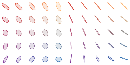
Bures--Wasserstein barycenters of centered Gaussian covariance matrices. Each panel shows a $5\times5$ grid of barycenter ellipses for four corner covariances, without separate input panels: the corner ellipses are the four input covariances themselves. The right grid uses more anisotropic inputs, making the nonlinear rotation and scaling of covariance barycenters more visible.

The interactive Gaussian demo compares the Bures covariance barycenter with a plain Euclidean covariance average under the same weights. The difference is most visible for rotated, anisotropic covariances: the Euclidean average blends matrix entries, whereas the Bures barycenter follows the geometry induced by quadratic Gaussian transport.

Sinkhorn for Barycenters¶

A key difference with the regularized two-marginal OT problem is that there is no canonical reference measure $\alpha\otimes\beta$, because the barycenter $\alpha$ is unknown. To reduce complexity, one usually fixes a candidate support for the barycenter and solves the discrete problem (1); this introduces a discretization error but keeps the number of unknowns manageable.

One can then use entropic smoothing and approximate (1) by

for some $\epsilon>0$. This is a smooth convex minimization problem, which can be tackled using gradient descent Cuturi & Doucet, 2014. An alternative is to use a descent method, typically quasi-Newton, on the semi-dual Cuturi & Peyré, 2016; this is useful when adding extra regularization on the barycenter, for instance to impose smoothness.

A simple but effective approach rewrites (10) as a weighted KL projection problem Benamou et al., 2015:

subject to

Here $K_s\eqdef e^{-C_s/\epsilon}$. The barycenter $a$ is implicitly encoded in the common row marginal

The optimal couplings have scaling form

and the generalized Sinkhorn iterations are

The geometric mean enforces the fact that all couplings share the same barycenter marginal.

Classical applications include two-dimensional image interpolation, three-dimensional shape interpolation, and barycenters on surfaces where the ground cost is the square of the geodesic distance Solomon et al., 2015.

Multimarginal OT¶

Multi-marginal OT couples more than two measures at once. It is the natural language for barycenters, matching with teams and several-body costs, but its tensor dimension is the main computational obstacle.

Definition and Basic Structure¶

The multi-marginal formulation replaces a coupling between two measures by a joint distribution with several prescribed marginals. Given measures $(\alpha_s)_{s=1}^S$ on spaces $(\X_s)_{s=1}^S$ and a cost $c:\X_1\times\cdots\times\X_S\to\RR$, the problem reads

where $\Couplings(\alpha_1,\ldots,\alpha_S)$ is the set of probability measures whose $s$-th marginal is $\alpha_s$. This is still a linear program in the discrete setting, but its ambient tensor has size $\prod_s n_s$.

Multi-Marginal Formulation of Barycenters¶

Wasserstein barycenters are the central example. For the squared Euclidean cost, one can introduce a latent barycenter point and eliminate it explicitly, leading to the multi-marginal cost

Entropic Regularization of Multi-Marginal OT¶

As in the two-marginal case, adding an entropic penalty with respect to the product measure $\alpha_1\otimes\cdots\otimes\alpha_S$ leads to scaling algorithms:

The optimizer has the generalized Gibbs form

and generalized Sinkhorn iterations alternately update one potential $f_s$ so that the $s$-th marginal is correct. The bottleneck is the tensor size $\prod_s n_s$ in the discrete case. Practical barycenter solvers exploit separability of the cost, low-rank structure, convolutional kernels, or a fixed barycenter support.

Metric Learning and Inverse OT¶

This section points to inverse problems where the ground cost itself is learned. Such problems are typically bilevel and non-convex, but OT provides useful gradients with respect to the cost.

Metric Learning and Derivatives of OT¶

OT is convex with respect to the measure and concave with respect to the cost. Ground-metric learning was explicitly studied in Cuturi & Avis, 2014, and it connects to the broader metric-learning literature Kulis, 2012Bellet et al., 2015.

Thus, if the cost is parameterized as $C_\theta$, gradients of losses involving OT values are obtained by backpropagating through the inner product $\dotp{P^\star(C_\theta)}{\partial_\theta C_\theta}$. The difficulty is not differentiating a solved OT problem, but learning a cost for which the resulting matching has the desired semantic behavior; this is a bilevel and usually non-convex optimization problem.

show_book_figure("metric-learning-cost-deformation")

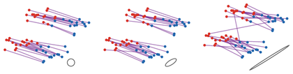
Changing the ground metric changes the optimal coupling. The same red and blue empirical measures are matched with $c_A(x,y)=(x-y)^\top A(x-y)$ for the Euclidean metric and two increasingly anisotropic Mahalanobis metrics. The small gray ellipse shows the unit ball of the metric: directions in which the ellipse is elongated are cheaper, and this deforms the transport segments selected by the OT plan.

The interactive demo lets the anisotropy and orientation of the Mahalanobis cost move. The transport plan is recomputed exactly for the displayed particles, so the segments show how the learned cost changes the matching.

Inverse Optimal Transport¶

Inverse OT asks for a ground cost that explains observed matchings or flows as optimal transport plans. In its most direct form, one observes a plan $\widehat\pi$ with marginals $(\alpha,\beta)$ and seeks a cost $c$ such that $\widehat\pi$ is optimal for

This is ill-posed without structure: adding potentials $u(x)+v(y)$ to a cost does not change the set of optimal couplings, and many costs can rationalize the same sparse plan.

A useful statistical methodology is to measure the suboptimality of the observed plan through a Fenchel--Young loss. Write the score as $s=-c$ and define the convex regularized prediction value

The Fenchel--Young loss

is nonnegative by Fenchel’s inequality and vanishes exactly when $\widehat\pi\in\partial G_\epsilon(-c)$, i.e. when $\widehat\pi$ satisfies the regularized optimality conditions for $c$. Entropic regularization is important here because it makes the forward map smoother and provides gradients with respect to $c$, at the price of a statistical bias Andrade et al., 2025Peyré et al., 2026.

In the discrete unregularized case, this loss reduces to the optimality gap of the observed coupling. For $\widehat P\in\mathbf U(a,b)$ and a cost matrix $C$, denote it by

This inverse-OT gap loss is nonnegative and vanishes exactly when $\widehat P$ is optimal for $C$.

In practice, one restricts the cost to a finite-dimensional model class, often affine:

where $\Theta$ is convex and the matrices $C^{(r)}$ encode features, graph distances or a Mahalanobis parameterization. This viewpoint appears in low-rank and sparse inverse OT models Dupuy et al., 2019Andrade et al., 2024 and in convex formulations for learning OT costs from observed plans Ma et al., 2020Peyré et al., 2026.

A minimal finite-dimensional model is obtained by learning a bilinear cost on $\RR^d$,

For empirical measures $\alpha=\frac1n\sum_i\delta_{x_i}$ and $\beta=\frac1n\sum_j\delta_{y_j}$, this gives the cost matrix

so both maps $A\mapsto C(A)$ and $A\mapsto c_A$ are linear. Inverse OT within this model asks which matrix $A$ makes an observed matching or coupling look optimal; learning the cost is thus reduced to estimating a linear parameter.

For a fixed matrix $A$, the forward prediction is the optimal face

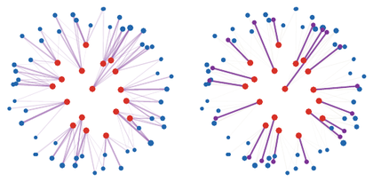
When this face is a singleton, write its element as $P_A$; otherwise $P_A$ denotes a deterministic tie-broken selection. Although $A\mapsto C(A)$ is linear, the solution correspondence $A\mapsto\mathcal P_A$ is polyhedral: changing $A$ changes the direction in which the transport polytope is probed, and a tie-broken selection is constant on normal-cone cells. The figure below illustrates this correspondence on the OT4ML point clouds. The construction follows the visual idea of the Python Optimal Transport logo Flamary et al., 2021: red source atoms, blue target atoms and straight segments show the selected optimal bijection. The rank-one matrices $A=-e_1e_1^\top$ and $A=-e_2e_2^\top$ only score horizontal or vertical correlations. The matrix $A=-I$ gives the usual quadratic $\Wass_2$ assignment, up to the marginal-only terms discussed below, while $A=+I$ reverses the correlation and produces an anti-$\Wass_2$ matching.

show_book_figure("inverse-ot-bilinear-logo-map")

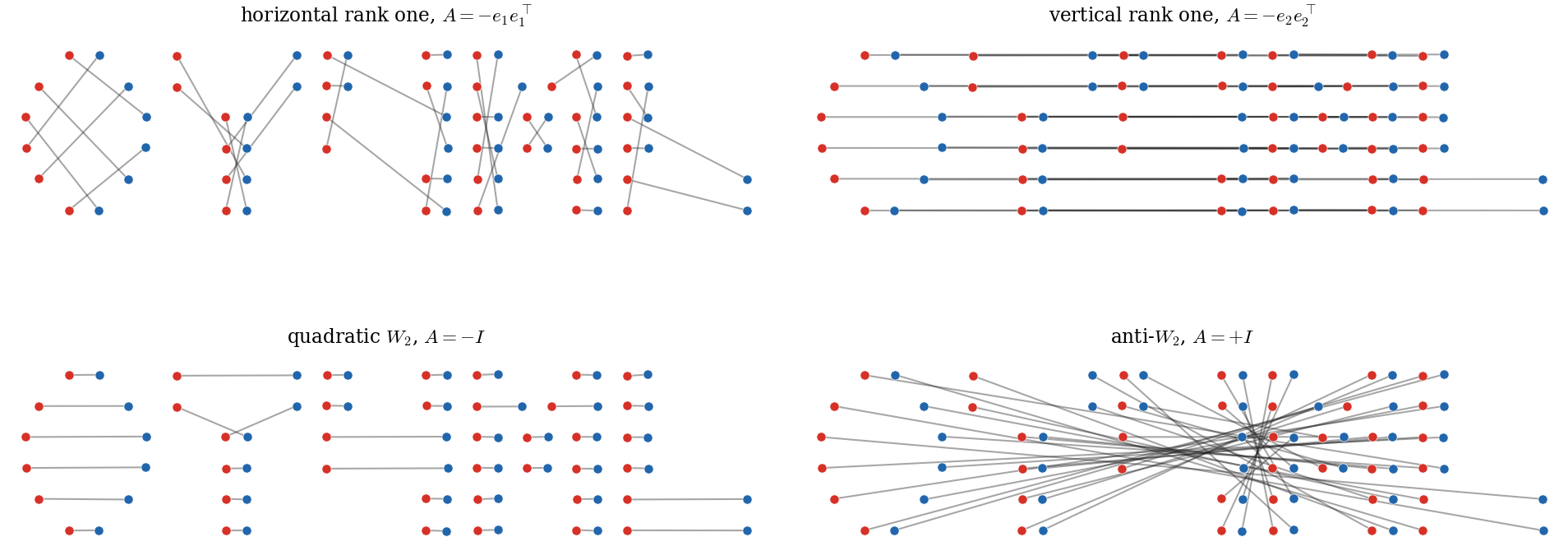
Forward solutions of the bilinear cost $c_A(x,y)=\dotp{Ax}{y}$ on the OT4ML logo point clouds. Each panel solves the equal-weight assignment problem with a different matrix $A$; the source atoms are red, the target atoms are blue, and the gray segments give one deterministic optimal bijection.

This elementary model already contains the quadratic Wasserstein assignment. Adding to a cost matrix a term depending only on $x_i$ or only on $y_j$ shifts all feasible couplings by the same constant, and therefore does not change the optimizer. Since

the usual quadratic Wasserstein assignment has the same optimizer as the bilinear cost with $A_\star=-I$, up to these marginal-only terms and an irrelevant positive factor. The inverse problem goes in the opposite direction: after observing a coupling, one asks which matrices $A$ could have generated it. The next figure generates an observed coupling $\widehat P$ from this cost on two empirical mixtures of Gaussians, and then evaluates $\mathcal L_{\mathrm{iOT}}(C(A_t);\widehat P)$ along the anisotropic path

so that $t=0$ recovers the matrix that generated the observed coupling. Equivalently, with equal weights, $\widehat P\in\CouplingsD(\ones_n/n,\ones_n/n)=\mathcal B_n/n$, and the plotted loss is the Kantorovich gap

Because $t\mapsto C(A_t)$ is affine and the Kantorovich value is a minimum of affine functions over the fixed polytope $\CouplingsD(\ones_n/n,\ones_n/n)$, this one-dimensional gap is convex and piecewise affine. Its zero set can contain an interval for a small sample, reflecting the fact that the same observed coupling remains optimal for a cone of nearby costs.

show_book_figure("inverse-ot-gap-loss")

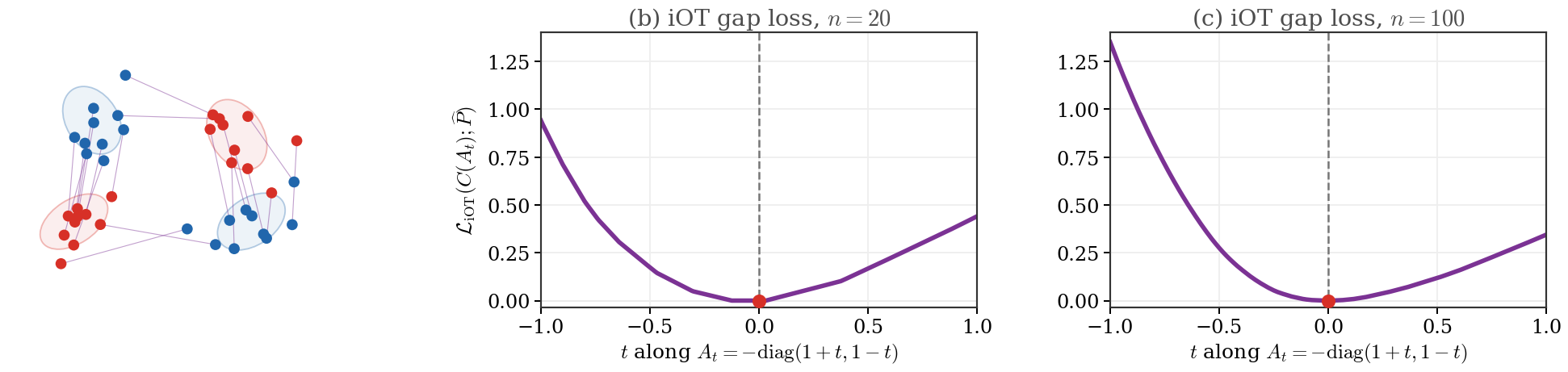
Inverse-OT gap loss for a bilinear cost. Panel (a): two empirical mixtures of two Gaussians are matched with the cost $c_{A_\star}(x,y)=\dotp{A_\star x}{y}$ for $A_\star=-I$, which gives the same optimizer as the quadratic $\Wass_2$ cost; red and blue level sets display the two sampling densities. Panels (b,c): the unregularized Fenchel--Young Kantorovich gap $\mathcal L_{\mathrm{iOT}}(C(A_t);\widehat P)$ along $A_t=-\diag(1+t,1-t)$ for $n=10$ and $n=100$, using the same vertical scale. The red dot marks the generating parameter $t=0$; the curves are convex and piecewise affine.

The comparison between $n=10$ and $n=100$ illustrates an important statistical effect: as the number of sampled points grows, the flat region of the empirical gap typically shrinks and the loss develops more visible curvature around the generating parameter. This anticipates the population theory of Peyré, Poon and Tron Peyré et al., 2026: in the limit $n\to+\infty$, when the limiting Monge map itself has nondegenerate curvature as the cost parameter varies, the iOT loss identifies the cost robustly, up to the usual marginal-only gauge freedoms. In that regime, minimizing the gap is not only a certificate of optimality of the observed transport, but also a stable way to recover the underlying cost.

The formulation is useful because it avoids differentiating through a forward OT solver: it learns a cost by making the observed plan satisfy complementary slackness. In statistical settings, $\widehat P$ is only partially observed or noisy, so one adds sparsity, low-rank, smoothness or metric constraints to select a meaningful cost. For entropic OT, the optimality condition becomes smoother:

which leads to likelihood-based or KL-based convex objectives when $C_\theta$ is affine, and connects inverse OT with generalized Sinkhorn iterations and transport-regularized inverse problems Karlsson & Ringh, 2016Ma et al., 2020.

Weak Optimal Transport¶

Weak OT relaxes the cost so that it depends on the conditional distribution of destinations rather than only on pointwise pairs. It is useful when a source point is allowed to choose a randomized response and the model only penalizes an aggregate of that response, such as its conditional mean.

Barycentric Projection of a Coupling¶

The first object to isolate is the map obtained by collapsing each conditional law to its barycenter.

The projected target $\bar\beta_\pi$ records the distribution of conditional means, not the full second marginal. Thus it is generally different from $\beta$; if $\pi=(\Id,T)_\sharp\alpha$ is induced by a map, then $\bar T_\pi=T$ and $\bar\beta_\pi=\beta$. This projection is not an optimal map for an arbitrary coupling: a deterministic rotation of a radially symmetric source, for example, projects to the rotation itself, whereas the optimal map from the source to itself is the identity. The useful positive statement is attached to quadratic optimal plans, as in the tangent-space viewpoint on $\Wass_2$ developed by Ambrosio, Gigli and Savare Ambrosio et al., 2006.

Weak transport costs use the same disintegration but allow the objective to depend on the whole conditional law, or on summaries such as the barycentric projection (46). The framework was introduced through general transport costs and weak transport inequalities, with existence, duality and optimality conditions developed on Polish spaces Gozlan et al., 2017Backhoff Veraguas et al., 2018. For a weak cost $C:\X\times\mathcal P(\Y)\to\RR\cup\{+\infty\}$, the weak OT value is

The classical Kantorovich problem is recovered when $C(x,\nu)=\int c(x,y)\d\nu(y)$, because the objective then becomes $\int c(x,y)\d\pi(x,y)$. The genuinely weak behavior starts when $C$ is nonlinear in $\nu$.

show_book_figure("weak-ot-barycentric-projection")

Weak barycentric transport on a small disk-to-annulus coupling. The left panel shows the full conditional laws: each red source atom splits its mass among several blue target atoms, with segment thickness proportional to transported mass. The right panel collapses each conditional law $\pi_x$ to its barycenter $\bar T_\pi(x)=\int y\d\pi_x(y)$, shown in violet. The barycentric weak cost only sees the red-to-violet displacement, and therefore ignores the conditional spread around each barycenter.

The interactive demo lets each source point split toward several targets. Increasing the split count or spread usually increases the full quadratic cost while the weak barycentric cost can remain much smaller.

The barycentric cost is the canonical example to keep in mind: admissibility still constrains the full conditional laws to have second marginal $\beta$, but the objective only charges the displacement from $x$ to $\bar T_\pi(x)$ and ignores the conditional variance around this barycenter. This connects weak OT with martingale transport, Strassen-type convex-order constraints, barycentric projections and learning problems where conditional averages are meaningful objects.